Use of Correlation Coefficient and Quartiles of Auxiliary Variable for Improved Estimation of Population Variance

(1)

Use of Correlation Coefficient and Quartiles of Auxiliary

Variable for Improved Estimation of Population Variance

Subhash Kumar Yadav1, S. S. Mishra1,*, Alok Kumar Shukla2

1

Department of Mathematics and Statistics (A Centre of Excellence), Dr. RML Avadh University, Faizabad, U.P., India

2

Department of Statistics, D.A.V College, Kanpur, U.P., India

Abstract

The present paper deals with the estimation of population variance using correlation coefficient and quartiles of an auxiliary variable under simple random sampling scheme. Up to the first order of the approximation, the bias and the mean square error of the proposed estimator have been obtained. The optimum value of the characterizing scalar kappa has been obtained and for this optimum value of kappa, the minimum mean square error of the proposed estimator has also been obtained up to the first order of approximation. A comparison of the proposed estimator has been made with existing estimators of population variance under simple random sampling scheme. An empirical study is also carried out to justify the theoretical findings. An improvement over existing estimators has been shown in the sense of having lesser mean square error.

Keywords

Ratio estimator, Quartiles, Bias, Mean squared error, Efficiency

1. Introduction

In survey sampling, auxiliary information is used for enhancing the efficiency of the estimate of the parameters of the population for the characteristic under study. Auxiliary information is supplied by the auxiliary variable which is highly positively or negatively correlated with the main variable under study. Ratio type estimators are used when the variables X and Y are positively correlated and the line of regression of y on x passes through origin, while the product type estimators are used when X and Y are negatively correlated to each other otherwise regression estimators are used. In the present study, we are dealing with only the positive correlation.

Let

( ,

x y

_i _i

),

i

=

1, 2,...,

n

be the n pair of observations for the auxiliary and study variables, respectively from the population of size N using simple random sampling without replacement. Let

X

and

Y

_be

the population means of auxiliary and study variables respectively and

x

and

y

be the respective sample means.

Following are the notations which have been used in this manuscript and are already being discussed by Subramani and Kumarpandiyan (2015) as:

N

: Size of the population

n

: Size of the sample

* Corresponding author:

[email protected] (S. S. Mishr)

Published online at http://journal.sapub.org/ajor

Y

: Study variable

X

: Auxiliary variable

ρ

: Correlation coefficient between

X

and

Y

X

Y

,

: Population means

x

y

,

: Sample means

2

y

S

,

S

_x2: Population variances

2

y

s

,

s

2_x: Sample variances

y

C

,

C

_x: Coefficient of variations

n

f

)

1 (

−

=

γ

n

f

N

=

2 / 02 2 / 20

s r

rs

_µ

µ

λ

=

1

1 (

) (

)

N

r s

rs i i

i

y

Y

x

X

N

µ

=

∑

−

3 02

2 03 ) (

1

_µ

µ

β

_x

=

: Skewness of the auxiliary variable

2 02 04 ) (

2

_µ

µ

β

_x

=

: Kurtosis of the auxiliary variable

1

Q

: First quartile of the auxiliary variable

3

(2)

r

Q

: Inter quartile range of the auxiliary variable

d

Q

: Semi quartile range of the auxiliary variable

a

Q

: Semi quartile average of the auxiliary variable

(.)

B

: Bias of the estimator

(.)

V

: Variance of the estimator

(.)

MSE

: Mean squared error of the estimator

100 *

)

(

)

(

)

,

(

p e p

e

t

MSE

t

MSE

t

PRE

=

: Percentage relative

efficiency of the estimator

t

_p over

t

_e

The appropriate estimator of the population variance is the sample variance defined as

2

0 y

t

=

s

, (1.1)

which is an unbiased estimator of the population variance and its variance up to the first order of approximation is given as

( )

4

(

)

0 40

1

y

f

V t

S

n

λ

−

=

−

, (1.2)

where

2 2 20 02

rs

rs r s

µ

λ

µ µ

=

,

1 1

( ) ( )

1

N

r s

rs i i

i

Y Y X X N

µ

=

= − −

−

∑

and

f

n

N

=

.

Isaki (1983) utilizing the auxiliary information, proposed the following classical ratio estimator for the population variance as

2 2

2

x R y

x

S

t

s





= 







, (1.3) where

2 2

1

1 (

)

1

n

y i

i

s

y

n

₌

=

−

∑

,

2 2

1

1 (

)

1

n

x i

i

s

x

n

₌

=

−

∑

,

2 2

1

1 (

)

1

N

x i

i

S

X

N

=

−

− =

∑

, 1

1 N

i i

X X N ₌ =

∑

,

1 1 N

i i

Y Y

N ₌

=

∑

,

1

n i i

x

n

₌

=

∑

,

1

n i i

y

n

₌

=

∑

.

The expressions for the Bias and Mean Square Error (MSE) of the estimator in (1.3) up to the first order of approximation respectively are as

[

]

2

40 22

(1

)

( )

_R

f

_y

(

1) (

1)

B t

S

n

λ

−

=

− −

−

, (1.4)

[

]

4

40 04 22

(1

)

( )

R y

(

1) (

1) 2 (

1)

f

MSE t

S

n

λ

−

=

− +

− −

−

, (1.5)

(Vide Kendall and Stuart (1977))

In the series of improvement, many authors have proposed different estimators of population variance utilizing the parameters of the auxiliary variable. Following table-1 which was also given by Subramani and Kumarpandiyan (2012) represents different estimators along with their bias, mean square error and constant.

Where symbols have their usual meanings.

C

x is the

coefficient of variation of auxiliary variable,

β

2(x) is the

coefficient of kurtosis,

Q

_i(i=1, 2, 3) are the quartiles of the auxiliary variable.

Q

_r,

Q

d and

Q

aare the functions of

quartiles defined by,

1

3

Q

_r

=

−

, Q_d =(Q₃−Q₁) 2,

Q

_a

=

(

Q

₃

+

Q

₁

)

2

. Thus, in general the mean square errors of the estimators given in above table may be written as,

[

(

1 )

(

1 )

2 (

1 )

]

)

ˆ

(

2( ) 22

2 )

( 2 4

2

=

λ

β

−

+

β

−

λ

−

i x

i y

y

i

S

R

S

MSE

(

i

=

1 ,

2 ,

...,

10

) (1.6) The latest references in the series of improvement can be made of Shukla et al. (2015) and Yadav et al. (2015a, 2015b, 2016).

Table 1. Bias, MSE and Constants of different estimators

Estimator Bias MSE Constant













+

=

x x

x x y

C

s

C

S

s

S

₂

2 2 2 1

ˆ

Kadilar and Cingi (2006a)













−

)

1 (

)

1 (

22 ) ( 2 1 1 2

λ

β

λ

x

y

R

S

    

  

− −

− +

−

) 1 ( 2

) 1 (

22 1

) ( 2 2 1 )

( 2 4

λ

β

λ

R R S_y y x

x x

x

C

S

R

+

=

₂ 2

1













+

=

) ( 2 2

) ( 2 2 2 2 2

ˆ

x x

x x y

s

S

s

S

β

Upadhyaya and Singh (1999)













−

)

1 (

)

1 (

22 ) ( 2 2 2 2

λ

β

λ

x

y

R

S

    

  

− −

− +

−

) 1 ( 2

) 1 (

22 2

) ( 2 2 2 )

( 2 4

λ

β

λ

R R S_y y x

) ( 2 2

2 2

x x

x

S

R

β

(3)













+

=

x x x x x x y

C

s

C

S

s

S

) ( 2 2 ) ( 2 2 2 2 3

ˆ

β

Kadilar and Cingi (2006b)













−

)

1 (

)

1 (

22 ) ( 2 3 3 2

λ

β

λ

x y

R

S

        − − − + − ) 1 ( 2 ) 1 ( ) 1 ( 22 3 ) ( 2 2 3 ) ( 2 4

λ

β

λ

R R S_y y x

x x x x x

C

S

R

+

=

) ( 2 2 ) ( 2 2 3

_β

β













+

=

) ( 2 2 ) ( 2 2 2 2 4

ˆ

x x x x x x y

C

s

C

S

s

S

β

Kadilar and Cingi (2006b)













−

)

1 (

)

1 (

22 ) ( 2 4 4 2

λ

β

λ

x y

R

S













−

+

−

)

1 (

2 )

1 (

)

1 (

22 4 ) ( 2 2 4 ) ( 2 4

λ

β

λ

R

S

_y y x

) ( 2 2 2 4 x x x x x

C

S

C

S

R

β

+

=













+

=

1 2 1 2 2 2 5

ˆ

Q

s

Q

S

s

S

x x y

Subramani and Kumarpandiyan (2012)













−

)

1 (

)

1 (

22 ) ( 2 5 5 2

λ

β

λ

x y

R

S

        − − − + − ) 1 ( 2 ) 1 ( ) 1 ( 22 5 ) ( 2 2 5 ) ( 2 4

λ

β

λ

R R S_y y x

1 2 2 5

Q

S

R

x x

+

=













+

=

3 2 3 2 2 2 6

ˆ

Q

s

Q

S

s

S

x x y













−

)

1 (

)

1 (

22 ) ( 2 6 6 2

λ

β

λ

x y

R

S













−

+

−

)

1 (

2 )

1 (

)

1 (

22 6 ) ( 2 2 6 ) ( 2 4

λ

β

λ

R

S

_y y x

3 2 2 6

Q

S

R

x x

+

=













+

=

r x r x y

Q

s

Q

S

s

S

₂ 2 2 2 7

ˆ













−

)

1 (

)

1 (

22 ) ( 2 7 7 2

λ

β

λ

x y

R

S

        − − − + − ) 1 ( 2 ) 1 ( ) 1 ( 22 7 ) ( 2 2 7 ) ( 2 4

λ

β

λ

R R S_y y x

r x x

Q

S

R

+

=

2 2 7













+

=

d x d x y

Q

s

Q

S

s

S

₂ 2 2 2 8

ˆ













−

)

1 (

)

1 (

22 ) ( 2 8 8 2

λ

β

λ

x y

R

S

        − − − + − ) 1 ( 2 ) 1 ( ) 1 ( 22 8 ) ( 2 2 8 ) ( 2 4

λ

β

λ

R R S_y y x

d x x

Q

S

R

+

=

₂ 2

8













+

=

a x a x y

Q

s

Q

S

s

S

₂ 2 2 2 9

ˆ













−

)

1 (

)

1 (

22 ) ( 2 9 9 2

λ

β

λ

x y

R

S

        − − − + − ) 1 ( 2 ) 1 ( ) 1 ( 22 9 ) ( 2 2 9 ) ( 2 4

λ

β

λ

R R S_y y x

a x x

Q

S

R

+

=

₂ 2

9













+

=

3 2 3 2 2 2 10

ˆ

Q

s

Q

S

s

S

x x y

_ρ

ρ

Khan and Shabbir (2013)

      − − − ) 1 ( ) 1 ( 22 ) ( 2 10 10 2

λ

β

λ

x y R R S         − − − + − ) 1 ( 2 ) 1 ( ) 1 ( 22 10 ) ( 2 2 10 ) ( 2 4

λ

β

λ

R R S_y y x

(4)

2. Proposed Estimator

Motivated by Prasad (1989) and Khan and Shabbir (2013), we propose an efficient ratio estimator of population variance as













+

=

3 2

3 2 2 2

ˆ

Q

s

Q

S

s

S

x x y

YM

_ρ

ρ

κ

, (2.1)

where

κ

_{is a suitable constant to be determined such that} the mean square error of

S

ˆ

_YM2 is minimum.

In order to study the large sample properties of the proposed estimator,

S

ˆ

_YM2 , we define

s

2_y

=

S

_y2

(

1 +

ε

₀

)

and

s

_x2

=

S

_x2

(

1 +

ε

₁

)

with

E

( )

ε

_i

=

0

for

(

i

=

0,1)

.

In case of simple random sampling without replacement, ignoring finite population correction term, the following

expectations could be obtained either directly or by the method due to Kendall and Stuart (1977) as

( )

2

(

)

0 40

1

f E

n

ε = − λ − ,

( )

2

(

)

1 04

1

f E

n

ε = − λ − ,

(

0 1

)

(

22

)

1

f E

n

ε ε

= −

λ

− .

Expressing

S

ˆ

YM2 in terms of

ε

i’s (

i

=

0 ,

1

), we have

1 1 10 0

2 2

)

1 )(

1 (

ˆ

₌

₊

−

e

R

e

S

_YM

κ

_y

After simplifying and retaining terms up to the first order of approximation, we have:

)

1 (

ˆ

2

1 2 10 1 0 10 1 10 0 2 2

e

R

e

R

e

R

e

S

YM

=

κ

y

+

−

+

Subtracting

S

_y2 on both the sides, we obtain,

2 2 1 2 10 1 0 10 1 10 0 2 2

2

)

1 (

ˆ

y y

y

YM

S

e

R

e

R

e

R

e

S

−

=

κ

+

−

+

−

(2.2) Taking expectation on both sides of (2.2), we have the bias of proposed estimator

S

ˆ

YM2 as:

[

(

1 )

(

1 )

]

(

1 )

)

ˆ

(

04 10 22 2

2 10 2

2

=

λκ

λ

−

λ

−

+

κ

−

y y

YM

S

R

S

B

(2.3)

where

(1

f

)

n

λ

=

−

.

The mean squared error of the proposed estimator

S

ˆ

YM2 is obtained by squaring both sides of (2.2), simplifying and taking

expectation on both sides, up to the first order of approximation as,

[

2

]

22 10 2

04 2 10 2

40 2 4 2

)

1 (

)

1 (

)

2 (

2 )

1 (

)

2

3 (

)

1 (

)

ˆ

(

S

=

S

κ

λ

−

+

κ

−

κ

R

λ

−

κ

−

κ

R

λ

−

+

κ

−

MSE

YM y (2.4)

)

ˆ

(

S

_YM2

MSE

is minimum for,

B

A

=

κ

(2.5)

where,

)

1 (

)

1 (

1

04 10 22

2

10

−

+

=

R

λ

R

λ

A

and

)

1 (

4 )

1 (

3 )

1 (

1 +

₄₀

−

+

₁₀2 ₀₄

−

₁₀ ₂₂

−

=

λ

R

λ

R

λ

B

The minimum MSE of the estimator

S

ˆ

YM2 for this optimum value of

κ

is:













−

=

B

A

S

MSE

_YM _y

2 4

2

min

(

ˆ

)

1

(2.6)

(5)

3. Efficiency Comparison

From (2.6) and (1.2), we have:

0 )

1 (

1 )

ˆ

(

)

(

₄₀

2 2

2 min

0



>











−

=

−

λ

B

A

S

MSE

t

V

_YM _y if

(

40

1 )

1

2

<

−

+

λ

B

A

(3.1)

{

(

1 )

(

1 )

2 (

1 )

}

0

1 )

ˆ

(

)

(

40 04 22

2 2

2

min



>











−

+

−

=

−

λ

B

A

S

MSE

t

MSE

R YM y

if

{

(

₄₀

1 )

(

₀₄

1 )

2 (

₂₂

1 )

}

1

2

<

−

+

−

+

λ

B

A

(3.2)

)

ˆ

(

)

ˆ

(

S

_i2

MSE

_min

S

_YM2

MSE

−

1

{

(

₄₀

1 )

2

(

₀₄

1 )

2 (

₂₂

1 )

}

0

2

_>













−

+

−

=

y

λ

R

i

λ

R

i

λ

B

A

S

, (

i

=

1 ,

2 ,

...,

10

)

if

{

(

1 )

2

(

₀₄

1 )

2 (

₂₂

1 )

}

1

40 2

<

−

+

−

+

λ

R

i

λ

R

i

λ

B

A

, (3.3)

4. Numerical Illustration

To justify the theoretical findings of different estimators, we have considered the following real populations. Population-1: Italian bureau for the environment protection-APAT Waste 2004

Y: Total amount (tons) of recyclable-waste collection in Italy in 2003. X: Total amount (tons) of recyclable-waste collection in Italy in 2002.

103 =

N

(Cities),

n

=

40

,

Y

=

626 .

2123

,

X

=

557 .

1909

,

ρ

=

0 .

9936

,

S

_y

=

913 .

5498

,

C

_y

=

1 .

4588

,

1117

.

818 =

x

S

,

C

_x

=

1 .

4683

,

λ

₀₄

=

37 .

3216

,

λ

₄₀

=

37 .

1279

,

λ

₂₂

=

37 .

2055

,

Q

₁

=

142 .

9950

,

6250

.

665

3

=

Q

,

Q

_r

=

522 .

6300

,

Q

d

=

261 .

3150

,

Q

a

=

404 .

3100

Population-2: Italian bureau for the environment protection-APAT Waste 2004 Y: Total amount (tons) of recyclable-waste collection in Italy in 2003.

X: Number of inhabitants in 2003.

103 =

N

,

n

=

40

,

Y

=

62 .

6212

,

X

=

556 .

5541

,

ρ

=

0 .

7298

,

S

_y

=

91 .

3549

,

C

_y

=

1 .

4588

,

1643

.

610 =

x

S

,

C

_x

=

1 .

0963

,

λ

₀₄

=

17 .

8738

,

λ

₄₀

=

37 .

1279

,

λ

₂₂

=

17 .

2220

,

Q

₁

=

259 .

3830

,

0235

.

628

3

=

Q

,

Q

_r

=

368 .

6405

,

Q

_d

=

184 .

3293

,

Q

_a

=

443 .

7033

. Population-3: Murthy (1967)

Y: Output for 80 factories in a region. X: Fixed capital.

80 =

N

,

n

=

20

,

Y

=

51 .

8264

,

X

=

11 .

2646

,

ρ

=

0 .

9413

,

S

y

=

18 .

3549

,

C

y

=

0 .

3542

,

4563

.

8 =

x

S

,

C

x

=

0 .

7507

,

λ

04

=

2 .

8664

,

λ

40

=

2 .

2667

,

λ

22

=

2 .

2209

,

Q

1

=

5 .

1500

,

975 .

16

3

=

Q

,

Q

_r

=

11 .

825

,

Q

d

=

5 .

9125

,

Q

a

=

11 .

0625

.

Population-4: Singh and Chaudhary (1986)

70 =

(6)

8572

.

140 =

x

S

,

C

_x

=

0 .

8037

,

λ

₀₄

=

7 .

0952

,

λ

₄₀

=

4 .

7596

,

λ

₂₂

=

4 .

6038

,

Q

₁

=

80 .

1500

,

0250

.

225

3

=

Q

,

Q

_r

=

144 .

8750

,

Q

d

=

72 .

4375

,

Q

a

=

152 .

5875

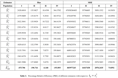
. Table 2. Bias and Mean square error of different estimators

Estimator Bias MSE

Population I II II IV I II II IV

2 1

ˆ

S

2420.6810 135.9827 10.4399 364.3702 67038384403 35796605 3850.1552 1415839

2 2

ˆ

S

2379.9609 135.8179 9.2918 363.9722 670169790 35796503 3658.4051 1414994

2 3

ˆ

S

2422.3041 135.9929 10.7222 364.4139 670393032 35796611 3898.5560 1415931

2 4

ˆ

S

2393.4791 135.8334 8.8117 363.8627 670240637 35796512 3580.8342 1414762

2 5

ˆ

S

2259.9938 133.4494 8.1749 359.3822 669558483 35795045 3480.5516 1427990

2 6

ˆ

S

1667.7818 129.8456 3.9142 350.4482 667000531 35792955 2908.6518 1408858

2 7

ˆ

S

1829.6315 132.3799 5.5038 355.3634 667623576 35794395 3098.4067 1419946

2 8

ˆ

S

2125.7591 134.1848 7.8275 359.8641 668911625 35795495 3427.1850 1429077

2 9

ˆ

S

1963.6570 131.6458 5.7705 354.8875 668182833 35793951 3133.3256 1418424

2 10

ˆ

S

1663.3086 127.6040 3.6276 348.1975 666910707 35791562 2878.5603 1398150

2

ˆ

YM

S

-475.706 -196.716 -6.168 -193.893 403977243 16417438 2078.2435 714592

Table 3. Percentage Relative Efficiency (PRE) of different estimators with respect to

t

₀

=

s

2_y

Estimator PRE

Pop-I Pop-II Pop-III Pop-IV

2

0 y

t

=

s

100.00 100.00 100.00 100.00

2 1

ˆ

S

573.93 107.48 140.03 92.76 2

2

ˆ

S

574.12 107.48 147.37 92.82 2

3

ˆ

S

573.92 107.48 138.30 92.76 2

4

ˆ

S

574.05 107.48 150.57 92.84 2

5

ˆ

S

574.63 107.49 154.91 91.98 2

6

ˆ

S

576.84 107.49 185.36 93.23 2

7

ˆ

S

576.30 107.49 174.01 92.50 2

8

ˆ

S

575.19 107.49 157.32 91.91 2

9

ˆ

S

575.82 107.49 172.07 92.60 2

10

ˆ

S

576.91 107.50 187.30 93.94 2

ˆ

YM

(7)

5. Observation and Conclusions

Table-1 shows the Bias, MSE and Constants for previously existing estimators given by different researchers. Proposed estimator which has been subjected to comparisons with previous estimators nothing but is a ratio estimator. In this paper, we have been able to develop more efficient estimator whose bias is significantly far much less as compared to previous estimators as evidently presented in table-2. Similarly, MSE is also far much less as compared to previous estimators given in the table-2. Moreover, table-3 shows that relative efficiency is comparatively much higher. Thus, we can finally conclude with passing remarks that from theoretical discussions in section-3 and the results in table-2 and 3, we infer that the proposed estimator is much better than the previously existing estimators of population mean in simple random sampling scheme, therefore proposed estimator should be preferred for the estimation of population variance.

ACKNOWLEDGMENTS

The authors are very much thankful to the editor of American Journal of Operational Research and the anonymous referees for critically examining the manuscript and giving the valuable suggestions to improve the manuscript in present form.

REFERENCES

[1] Isaki, C, T., (1983). Variance estimation using auxiliary information, Journal of American Statistical Association, 78, 117- 123.

[2] Kadilar, C. and Cingi, H., (2006a). Improvement in variance estimation using auxiliary information, Hacettepe Journal of mathematics and Statistics, 35, 111-15.

[3] Kadilar, C. and Cingi, H., (2006b). Ratio estimators for population variance in simple and Stratified sampling, Applied Mathematics and Computation, 173, 1047-1058. [4] Kendall, M. and Stuart, A., (1977). The advanced theory of

statistics, Vol I, Charles Griffin & Co., London.

[5] Khan, M. and Shabbir, J., (2013). A Ratio Type Estimator for the Estimation of Population Variance using Quartiles of an Auxiliary Variable, Journal of Statistics Applications & Probability, 2, 3, 319-325.

[6] Murthy, M. N., (1967). Sampling Theory and Methods, Statistical Publishing Society Calcutta, India.

[7] Prasad, P. (1989). Some improved ratio type estimators of population mean and ratio in finite population sample surveys, Communications in Statistics: Theory and Methods, 18, 379-392.

[8] Reddy, V., (1973). On ratio and product methods of estimation’, Sankhya Serie B 35(3), 307–316.

[9] Reddy, V., (1974). On a transformed ratio method of estimation’, Sankhya Serie C 36, 59–70.

[10] Singh, D. and Chaudhary, F. S., (1986). Theory and analysis of sample survey designs, New-Age International Publisher. [11] Shukla, A.K, Misra, S., Mishra, S.S. and Yadav, S.K (2015). Optimal Search of Developed Class of Modified Ratio Estimators for Estimation of Population Variance, American Journal of Operational Research, 5, 4, 82-95.

[12] Singh, H. and Karpe, N. (2010). Estimation of mean, ratio and product using auxiliary information in the presence of measurement errors in sample surveys’, Journal of Statistical Theory and Practice 4(1), 111–136.

[13] Singh, H. and Kumar, S., (2008). A general family of estimators of finite population ratio, product and mean using two phase sampling scheme in the presence of non-response’, Journal of Statistical Theory and Practice 2(4), 677–692. [14] Singh, H. and Vishwakarma, G., (2008). Some families of

estimators of variance of stratified random sample mean using auxiliary information, Journal of Statistical Theory and Practice 2(1), 21–43.

[15] Srivenkataramana, T. and Tracy, D. (1980). An alternative to ratio method in sample surveys’, Annals of the Institute of Statistical Mathematics 32, 111–120.

[16] Subramani, J. and Kumarapandiyan, G. (2012). Variance estimation using quartiles and their functions of an auxiliary variable, International Journal of Statistics and Applications, 2, 67-72.

[17] Subramani, J. and Kumarapandiyan, G. (2015). A class of modified ratio estimators for estimation of population variance. Jamsi, 11, 1, 91-114.

[18] Upadhyaya, L.N. and Singh, H.P. (1999). An estimator for population variance that utilizes the kurtosis of an auxiliary variable in sample surveys, Vikram Mathematical Journal, 19, 14-17.

[19] Yadav, S.K., Kadilar, C., Shabbir, J. and Gupta, S. (2015a). Improved Family of Estimators of Population Variance in Simple Random Sampling, Journal of Statistical Theory and Practice, 9, 2, 219-226.

[20] Yadav, S.K., Mishra, S.S., Shukla, A.K. and Tiwari, V. (2015b). Improvement of Estimator for Population Variance using Correlation Coefficient and Quartiles of The Auxiliary Variable, Journal of Statistics Applications and Probability, 4, 2, 259-263.

[21] Yadav, S.K., Misra, S. and Mishra, S.S. (2016).

Efficient Estimator for Population Variance Using Auxiliary Variable, American Journal of Operational Research, 6, 1, 9-15.