A Tabu Search Method for a New Bi-Objective Open Shop Scheduling Problem by a Fuzzy Multi-Objective Decision Making Approach (RESEARCH NOTE)

RESEARCH NOTE

A TABU SEARCH METHOD FOR A NEW BI-OBJECTIVE OPEN

SHOP SCHEDULING PROBLEM BY A FUZZY

MULTI-OBJECTIVE DECISION MAKING APPROACH

O. Seraj and R. Tavakkoli-Moghaddam*

Department of Industrial Engineering and Center of Excellence for Intelligence Based Experimental Mechanics College of Engineering, University of Tehran, P.O. Box 11155-4563, Tehran, Iran

[email protected] - [email protected]

*Corresponding Author

(Received: November 25, 2008 – Accepted in Revised Form: July 2, 2009)

Abstract This paper proposes a novel, bi-objective mixed-integer mathematical programming for an open shop scheduling problem (OSSP) that minimizes the mean tardiness and the mean completion time. To obtain the efficient (Pareto-optimal) solutions, a fuzzy multi-objective decision making (fuzzy MODM) approach is applied. By the use of this approach, the related auxiliary single objective formulation can be achieved. Since the OSSP are known as a class of NP-hard problems, a tabu search (TS) method is thus used to solve several medium to large-sized instances in reasonable runtime. The efficiency of the results obtained by the proposed TS for small, medium and large-sized instances is evaluated by considering the corresponding overall satisfactory level of all objectives. Also the adaptability of the yielded solutionsof the proposed TS for the small-sized instances is evaluated by comparing the results reported by the Lingo software. Several experiments on different-sized test problems are considered and the related results are indicated the ability of the proposed TS algorithm to converge to the efficient solutions.

Keywords Open Shop Scheduling Problem, Fuzzy Multi-Objective Decision Making, Tabu Search

!" #$% &

'( )

* ( +,- # ./

'0 1! 2

3!-'( 4 " !- - 4

!- 5678 9:

.

9: <.= - !

) .8? )@ (

B6C8 7" )D ,

+E$: ( ! ./

.

F 7" 8

#G8 ! &

. !)D H

9: 0 . '0 ( = -& '( )

= ( "

.I J )D 6= ( '0 5K 9: F 9%: J

'( L " #:.$

@)M? N.)6 .O$= P" Q) ./

. P" <.= - ' !

5*

+( ( L " #:.$ D.- ! : RS

9: - Q: T$ +0

U. 1! V.8 ( <.= !

./ . <.= WGQ 9X )Y6! !

9: ( +0

P"

( 5* J

( RS

& '0 <.= ! Z ( 5K !

: .4) ./

. [$

( " : +( C8 5* ( F8 "

\"E$ ! 'M

- ! @)M? B$.4

N.)6 .O$= 46! ] .8

<.= '/ ^ !

<.T ) ( .

1. INTRODUCTION

Assigning or sequencing some activities which require to be processed through a set of limited available resources (instance machines) is called scheduling. Efficient scheduling helps us to increase the efficiency of the capacity utilization by reducing

order of any job processing. In other words, the order of jobs processed on a machine, and the order of machines to process a job can be selected arbitrarily. Usually the goal of the OSSP is to find a feasible combination of the order of machines and jobs (i.e., a feasible schedule) in order to minimize the makespan that is also known as overall completion time in dynamic scheduling, in which the ready times are not zero. With this ordering constraints relaxed from a job shop problem, it results in a larger space of the OSSP structure.

The OSSP seems to get less attention from researchers. It has a larger solution space than the job shop or flow shop scheduling problems. Thus to achieve good solutions in reasonable computation time, applying a number of meta-heuristics might be useful in such a hard problem. The OSSP has many applications in industry and manufacturing systems. For example consider a large automotive garage, in which each vehicle may need some activities, such as replace exhaust pipe, align the wheels and tune up. These activities should be done for one job, and can be performed in any order. This problem is a class of NP-hard problems [1]. The OSSP may use in testing facilities where activities should not be done in any specified order which frequently applied in testing the elements of an electronic system. In general, this problem can be used in order to repair facilities in an arbitrary order [2].

Brucker, et al [3] and Liaw [4] proposed exact solution methods which followed by branch-and-bound and elimination methods to obtain an optimal solution. Tavakkoli-Moghaddam, et al [5] developed a new mathematical model for parallel machines scheduling problems with sequence-dependent setup times and precedence constraints to minimize the number of tardy jobs and total completion time of all jobs. As mentioned before, finding optimal solutions for medium or large-scale OSSP needs the vast amount of computational times, thus it is not a practical choice. Some meta-heuristics, which are widely used in scheduling problems, are an ant colony optimization (ACO) algorithm [6] for a flow shop scheduling problem, a simulated annealing (SA) method [7] for an open shop problem, a tabu search (TS) method [8,9] for the OSSP, a genetic algorithm (GA) [10] for a flow shop scheduling problem. A genetic algorithm (GA)

[11] proposed for a parallel machine scheduling with family setup times. In addition, some researchers applied hybrid heuristics, such as hybrid genetic algorithms (HGAs) [12-15] for job shop scheduling problems, a HGA [16] for a flow shop scheduling problem, and a HGA [17] for the OSSP.

In this paper, the discussion is focused on the open shop scheduling problems, and a mathematical formulation is also introduced. To solve some large-scale problems, a tabu search method is also proposed to obtain near-optimal solutions in a little computational time.

The rest of this paper is organized as follows. The static scenario taken into consideration in the model construction is described in Section 2. The related mathematical formulation is developed in Section 3, followed by the proposed fuzzy MODM method in Section 4. An efficient TS method is presented in Section 5. Computational results of small, medium and large-sized numerical experiments are given in Section 6. At last the deductions of this study and possible future researches are presented in Section 7.

2. PROBLEM DEFINITIONS AND ASSUMPTIONS

Most of the scheduling problems are associated with n jobs on m machines. If ni be the number of operations to be performed on machine i, then for an n job, m machine scheduling problems there are (n1)!(n2)! ... (nm)! Theoretically possible sequences which not all of them are feasible. The best sequence should be technologically feasible and optimizes the effectiveness measure. Considering the job operational flow or the processing order, n job on m machine scheduling problems can be divided into four categories as follows: flow shop, job shop, dependent shop, and open or general shop.

shop is called a general or open shop. Thus the open shop system has much flexibility in scheduling; however, it is difficult to develop a rule that give an optimal sequence for each problem [18].

The assumptions considered in this paper are listed below:

• Each of n jobs should be processed on m or fewer machines.

• Each job follows an arbitrary machining order and has a specified processing time. • Each job has a certain due date.

• One of the considered objectives in described OSSP is to minimize the mean completion time.

• Another objective is to minimize the mean of job tardiness. Let these two objectives have the same importance in making a decision.

• All n jobs are simultaneously available at the beginning of the planning period.

• A single job cannot be processed

simultaneously by more than one machine. • The processing time for each job on each

machine is known.

• Setup times and transportation times are independent of the sequence and are included in the processing times for all jobs. • The importance level of all jobs is assumed

to be equal.

• All m machines are available at the beginning of the planning horizon and ready to work on any of n jobs which require that machine.

• At any given time, at the most one job can be processed on a specific machine.

• There is only one machine of each type in the shop.

• In-process inventory is not allowed, i.e. the jobs cannot have the waiting time.

• The removal times and transportation times are assumed to be zero for all jobs in the shop.

• In this study it is assumed that preemption is not allowed that is, any started operation must be completed without interruptions. • Operations of a job can be processed in any

order.

The following section contains a list of symbols and their definitions used in this paper. In addition, a mixed-integer programming model is formulated for the above-mentioned scenario that is presented in the next section.

3. MATHEMATICAL MODEL

In this section, the described bi-objective open shop scheduling scenario is treated as a mixed-integer mathematical formulation. The notations, parameters, and decision variables are described as follows.

3.1. Model Notations To describe the addressed OSSP, the following notations are used:

i, j Job indices (i, j = 1,…,n). k, l Machine indices (k, l = 1,…,m). Oik Operation of job i on machine k (i =

1,…,n; k = 1,…,m).

M A large positive number.

di Due date of job i (i = 1,…,n).

pik Processing time of job i on machine k (i = 1,…,n; k = 1,…,m).

stik Starting time of processing job i on machine k (i = 1,…,n; k = 1,…,m). Cik Completion time of job i on machine

k (i = 1,…,n; k = 1,…,m).

xijk If job i precedes job j on machine k, then xijk = 1; Otherwise, xijk = 0 (i, j = 1,…n; k = 1,…,m)

yikl If job i on machine k precedes the same job on machine l, then yikl = 1; Otherwise, yikl = 0 (i = 1,…,n; k, l = 1,…,m).

3.2. Mathematical Formulation The mixed- integer mathematical programming has been formulated as follows:

       

×

     

=

∑

= n

i i T n

Z

1 1

1

min (1)

    

  

×

     

×

=

∑∑

= =

n

i m

k ik C m

n Z

1 1 2

1

s.t.

k i T d p

st_ik+ _ik− _i ≤ _i ;∀, (3)

k i C p

st_ik+ _ik≤ _ik ;∀, (4)

(

y

)

st i k l

M p

st_ik+ _ik− × 1− _ikl ≤ _il ;∀ , , (5)

l k i st y M p

st_il+ _il− × _ikl ≤ _ik ;∀ , , (6)

(

x

)

st i j k

M p

stik+ ik− ×1− ijk ≤ jk ;∀, , (7)

k j i st x M p

stjk+ jk − × ijk ≤ ik ;∀, , (8)

k j i x

x_ijk + _jik =1;∀, , (9)

l k i y

y_ikl + _ilk =1;∀ , , (10)

{

}

i j k

x_ijk∈ 0,1 ;∀ , , (11)

{

}

i k l

y_ikl∈ 0,1 ;∀, , (12)

k i

C_ik ≥0;∀, (13)

i

Ti ≥0;∀ (14)

3.3. Model Descriptions The objective (1), seeks to minimize the mean job tardiness. Objective (2) attempts to minimize the mean job completion time. Constraint (3) describes the tardiness for each job which defines as:

{ }

C d i n

T _{ik i}

m k

i max 0, max ; 1,2,...,

, . . . , 2 , 1

=

   

 

− =

= (15)

Constraint (4) considers the relation between starting processing time, processing time, and completion time in the shop. Constraints (5) and (6) indicate the relationship between each two consecutive operations (machines) of a job. Constraints (7) and (8) express the precedence between each pair of jobs on each related machine. Constraint (9) specifies the order relation between two jobs on a machine. Constraint (10) determines the order relation between two consecutive operations (machines) of a job. Constraints (11) to (14) represent integrality and non-negativity conditions.

4. FUZZY MULTI-OBJECTIVE DECISION MAKING APPROACH

Several approaches for solving multi-objective linear programming (MOLP) models are presented in the literature. Most of these approaches are fuzzy programming methods. A brief review of these methods is presented in the following paragraph. For more details refer to Torabi, et al [17].

The first fuzzy approach for solving a MOLP developed by Zimmermann [20] is called max–min approach; however the solution yielded by a max– min operator is well-known that may neithr be unique nor efficient [21-22]. Thus, thereafter to remove this deficiency several methods are proposed. Particular interests are the augmented max–min approach (LH method) [22], a modified version of Werners’ approach [23] (MW method) [24], a two-phase fuzzy approach (LZL method) [25], and a fuzzy approach (TH method) [19]. The TH method is a combination of LH and MW methods. Each of the TH, LH and MW methods usually gives us the efficient solutions of an MOLP model. Moreover they are more flexible than the LZL approach, also due to their single-phase characteristic [19]. Thus, we evaluate TH, LH and MW methods by applying them to several small-sized test problems generated at random. The obtained results indicate that all of these three methods always yield the efficient (non-dominated) solutions (i.e., an efficient solution is a feasible solution if there is no other feasible solution that yields an improvement in one objective without causing degradation in at least one other objective). The TH method, which is a combination of the LH and MW methods, yields several options for an MOLP because of its parameters combinations. In addition, The TH and MW methods propose more flexible formulation of an aggregation function. However, the LH method can be a suitable method along with the TH method. In this case, the LH method not only yields an efficient solution in a few runtime, but also is easier to apply in the proposed tabu search algorithm. Thus in this paper, the proposed bi-objective mixed integer model is solved by using the LH method.

following steps convert this model to a single-objective mixed-integer formulation.

Step 1. For each objective function calculate the positive ideal solution ( PIS

k

Z ) and negative ideal

solution (ZkNIS) by the following equations. Assume that, F be a set of all model constraints (i.e., Constraints (3) to (14)).

F T n Z n i i PIS ∈ Χ         ×       =

∑

= s.t. 1 min 1 1 (16) F T n Z n i i NIS ∈ Χ         ×       =

∑

= s.t. 1 max 1 1 (17) F C m n Z n i m k ik PIS ∈ Χ         ×       × =

∑∑

= = s.t. 1 min 1 1 2 (18) F C m n Z n i m k ik NIS ∈ Χ         ×       × =

∑∑

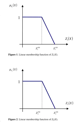
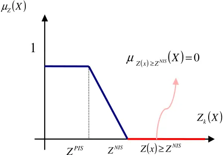
= = s.t. 1 max 1 1 2 (19)

Step 2. Define a linear membership function for each obtained positive and negative objectives in Step 1, use the following membership equations. Suppose that

( )

X

k

Z

µ

be the satisfaction level of the k-th objective for decision vector X (see Figures 1 and 2).

( )

       ≤ ≤ − − > = otherwise 0 , 1 2 1 2 1 1 1 1 1 2 1 Z Z Z Z Z Z Z Z Z

X iNIS

PIS i PIS NIS NIS PIS i Z µ (20)

( )

       ≤ ≤ − − > = otherwise 0 , 1 2 2 2 2 2 2 2 2 2 2 Z Z Z Z Z Z Z Z Z

X NIS PIS PIS NIS

NIS

PIS

Z

µ (21)

Step 3. Convert the bi-objective model to its related equivalent single-objective model by using LH aggregation functions and their corresponding formulations.

Equations 22 to 28 show that how the aggregation functions of the LH method can be inserted to the final crisp MOLP model. The LH aggregation function is used in subsequent model. Consequently the auxiliary single-objective model for the OSSP is obtained.

( )

∑

( )

= + = 2 1 Zk max k k X

X λ δ θ µ

λ (22)

( )

X

Z₁

µ

( )

X Z₁ PIS Z1 NIS Z1

1

Figure 1. Linear membership function of Z1(X).

( )

X

Z2 µ

( )

X Z₂ PIS Z2 NIS Z2

1

s.t.

(

NIS PIS

)

n

i i NIS

Z Z

T n

Z

1 1

1 1

1

− × ≥

       

×

     

−

∑

=

λ

(23)

(

NIS PIS

)

n

i m

k ik NIS

Z Z

C m

n Z

2 2

1 1 2

1

− × ≥

    

  

×

     

×

−

∑∑

= =

λ

(24)

F

∈

Χ (25)

1

2

1

=

∑

=

k k

θ (26)

2 , 1 ,

0 =

> k

k

θ (27)

[ ]

0,1 ∈

λ (28)

Where δ _{is a small positive number adequately} which is usually set to 0.01 [21,22]. Moreover, the preferences of the objectives are determined by the decision maker as: θ_{1 =} θ_{2, thus the objectives} weight vector is set to θ_{1 =} θ_{2 = 0.5. Take notice, F} is the set of Constraints (3) to (14).

Since the OSSP has a large solution space, thus to achieve a good solution in reasonable computation time for some large-scale problems, a tabu search (TS) method is proposed in the next section.

5. PROPOSED TABU SEARCH

The tabu search (TS) method was first defined and introduced by Glover [26,27], which is an individual local search-based method for solving hard combinatorial optimization instances. Following is a brief description of the TS method. In the first step, a move function must be defined to transform a solution to another one. For instance, a move function can replace some jobs in a basic sequence. With such a function, this method can generate some new solutions from a basic (or initial) sequence. Therefore, with the move function, the TS search through the neighborhood of an initial solution in order to find the best sequence around its local area. After that, the method repeats the

neighborhood search procedure from the obtained best sequence, as a new basic solution in decision space, and the process will be continued. Moreover, the system of a tabu list is introduced to avoid cycling. The components of the tabu list indicate the current tabu moves (i.e., the forbidden sequences in the current neighborhood search are determined by these elements). When the TS find a new basic sequence in the neighborhood search procedure, the oldest element of the tabu list should be exchanged with the related new one. The search procedure stops when a stop criterion holds. The design of the TS components influences the performance of the TS, convergence speed, or its running time.

5.1. Initial Solution Various methods can be applied to yield an initial solution, such as a related priority dispatching rule or a random method. We apply a random method to several numerical experiments in different sizes. The results expressed a little influence of the random method on the quality of the solutions. Thus, we use the random method to generate the initial solution (as a basic sequence) as follows. Since we consider n jobs and m machines in the OSSP, each feasible point of the solution space is connected to an n × m array of operations Oik. Thus, we yield the random basic sequences through generating a random permutation of Oikin an n×moperation-based array.

5.2. Moves and Neighborhood As mentioned before, a function which transforms a sequence to another sequence in the current neighborhood, called a move function. Since the neighborhood structure directly affects on the performance of the algorithm, the infeasible moves not allowed in our search and unnecessary moves were eliminated too. Three types of move functions have been considered in the literature:

• Swap each two adjacent jobs that are placed at the positions p and (p+1); p = 1, 2,...,n × m, in the above-mentioned operation-based array.

• Swap two jobs that are placed at the positions p and p′_{; p, p}′ _{= 1,2,...,n × m, in the}

related operation-based array.

• Remove a job that is placed at the p-th position and insert it to the p′_{-th position of}

After applying these move types to some random test problems, we choose the first move type in our proposed TS, because of its feasibility adaptation and solution diversification.

5.3. Move Evaluation The yielded solution from each move is evaluated as follows. As mentioned before, each feasible sequence of the solution space considered as an n × m operation-based array. Since moves yield feasible arrays, thus for evaluating each array, at first an n × m completion time matrix with zero elements is defined. Considering the order of arranged operations Oik in an array, we start calculating from position one (p=1), then go to position two (p=2), and finally continue to position n × m (p= n×m). Thus, each element of the related completion time matrix can be calculated as:

{ }

{ }

_

 

+ =

=

= n ik k m ik

i p

ik p

ik p c c

c

., . . , 2 , 1 ,

. . . , 2 ,

1 , max

max

max (29)

With these completion times, the mean job tardiness and mean completion time can be computed. Furthermore, applying the proposed Equations 19 and 20, µZ₁

( )

X and µZ₂

( )

X can be computed as

well. To calculate the overall satisfactory level (λ), the following system of inequalities should be solved:

( )

( )

[

]

    

∈ ≥ ≥

1 , 0

2 1

λ

λ µ

λ µ

X X

Z Z

(30)

Since only λ is unknown in this system, thus we can calculate λ as follows:

( )

( )

{

_Z X _Z X

}

2 1 ,

min µ µ

λ = (31)

Consequently the above calculated parameters are located into the aggregation function of the LH method. The obtained value is used to evaluate the related move. A move with the greatest value of the LH aggregation function is the best move in the current neighborhood.

5.4. Tabu List In the search procedure, there may exist some moves that bring the TS method back to recently obtained solutions. These moves

should be considered as tabu moves for a certain number of iterations. Thus the characteristics of these moves must be kept in a list, called a tabu list. To update the tabu list, when the TS finds a best sequence in a neighborhood, the associated characteristics of this move should be exchanged with the oldest element of the tabu list. The size of the tabu list is an important parameter, because a large tabu list may restrict the search procedure and a small tabu list may lead to cycling risk. The size of the tabu list is usually selected from the set {5-9}. We applied these sizes of the tabu list to some test problems with different sizes. Considering the yielded results, the size of tabu list for small and medium to large-sized problems is set to 5 and 7, respectively.

5.5. Stopping Criteria In general, there are three stopping criteria commonly used in the literature:

• The obtained best sequence is close enough to a lower bound of the optimum value. • The number of iterations without any

improvement in the objective function value passes a specified limit.

• The computational time or total number of iterations passes a certain restriction.

Two latter stopping criteria are simultaneously applied in our proposed TS method.

6. NUMERICAL EXPERIMENTS

In this section, several numerical instances with different combinations of jobs and machines are generated randomly in small, medium, and large sizes in order to evaluate the performance of the

proposed TS method and fuzzy MODM

even after several hours running. However, fortunately the Lingo can yield a feasible solution for these instances in reasonable run time, which can help us to construct the related positive and negative ideal solutions. Also, for all instances the TS method is coded in MATLAB R2008a on a 32-bit operation system with Intel(R) core(TM) 2 Duo CPU 2.2 GHz and 2038 MB of RAM VAIO computer.

6.1. Instances Generation In the literature there is a classical method to generate the numerical instances of n|jobs and m|machines scheduling problems randomly [28]. This method is implemented as follows. The processing times and due dates are uniformly distributed in the

intervals [0,100] and 

  

 

   

 

+ −

   

 

− −

2 1 , 2

1 T R P T R

P ,

respectively. In this formulation, two parameters R and T are taken into consideration in the sets {0.2, 0.6, 1.0} and {0.4, 0.6, 0.8}, respectively. Also in the case of n|jobs and m|machines scheduling, we have |P=

(

m+n−1

)

p, where p is the mean of total processing times.

Considering this instance generating method, the number of jobs can be 4 to 6, and the number of machines can be 2 to 4 for small-sized problems. Also for medium and large-sized problems, the number of jobs can be 10, 12, 15, and 30, and the number of machines can be 6 to 9. For each of these random instances, the manufacturing system is defined as a number of jobs|×|number of machines, for example the problem 10 × 6 indicates a manufacturing environment with 10 jobs and 6 machines.

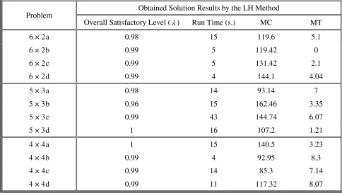
6.2. Defining The Positive and Negative Ideal Solutions As mentioned before, in the proposed fuzzy MODM approach, a linear membership function is considered for each objective. Therefore, we can define an uncertain boundary for each membership function as

[

iNIS

]

PIS

i Z

Z , . On the

other hand, let X denotes a decision vector is solution space. In this case ∀x∈X if _Z

( )

_{x <Z}PIS_, the membership value of x will be greater than zero. Thus, x will be taken into consideration in the related fuzzy MODM aggregation function. Since the MODM algorithm defines a membership value

for each point of solution space, if the membership value of a feasible solution is equal to zero, that point will not be considered in the algorithm any more (see Figure 3). Therefore, if we choose a large/small value for ZNIS, the diversity of yielded solutions (x∈X ) in our proposed TS will increase/decrease, because the large/small values of ZNIS increase/decrease the

[

NIS

]

i PIS

i Z

Z , interval

with the fixed amount of ZPIS.

To yield the ZPIS and ZNIS, each generated test problem is solved, according to the presented Equations 16 to 19. This is clear that for all test problems the obtained value of the ZkNIS will be unbounded, thus we consider the subsequent heuristic method which considered in literature [19,22]. Let Xi denotes the associated decision vector with the ZiPIS (i.e., positive ideal solution of

the i-th objective); the related NIS k

Z can be

estimated as follows: max

{

( )

}

; 1,2

2 , 1

= =

= Z X k

Z _i i

i NIS

k .

However after some experiments, we find out in the OSSP that this method not only yields a small value for NIS

k

Z , but also requires more

computational times and limit the search procedure greatly. Therefore, we consider the following heuristic formulations. The formula MCPIS

NIS

MC Z

Z =3×

is being applied to small-sized problems, also PIS

MC NIS

MC Z

Z =4× is being studied for medium and

large-sized instances optionally for the mean completion time objective to cover several

( )

X

Z

µ

PIS

Z ZNIS

1

( )

X Z_k

( )

_{x Z}NIS

Z ≥

( )_x≥_ZNIS

( )

X =0

Z

µ

solutions in the feasible decision space. Similarly,

(

m n

)

Z

Z_MTNIS = _MTPIS + + is also being considered for

the mean tardiness objective in all instances. The number of jobs and machines are inserted into the latter formula to connect that to the size of instances. The results of several experiments show that these proposed values of ZNIS, either do not limit the search algorithm, or do not increase the solution time widely.

Since for medium and large-sized problems ZPIS cannot be obtained in a reasonable runtime, because they are time-consuming instances (e.g., for a 10 × 6 problem), the Lingo cannot yield the ZPIS after 7 hours running. But fortunately, for these problems, the Lingo can give us a feasible solution with its objective value in a few minutes. Thus, in our study, the Lingo is run several times for each medium and large-sized instance. Consequently for each of them some different feasible solutions are yielded. Since for these instances, the objective functions of their related feasible solutions are known, the minimum value them is selected for their corresponding ZPIS (see Tables 1 and 2).

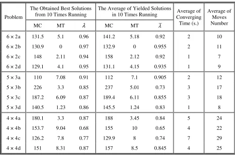
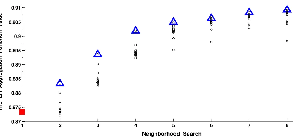
6.3. Solution Quality and Efficiency We can evaluate the solutions efficiency by considering the overall satisfactory level (λ) of all objectives yielded from the LH method. For example the λ ₌ 0.9 for an obtained solution, indicates that in the current solution all of the objectives are satisfied 90 percent. Thus the greater values of λ denote the higher degree of the efficiency. Moreover in small-sized instances, the quality of an obtained solution from our proposed TS method can be evaluated by making a comparison with the yielded optimal solution. The obtained solutions from the Lingo and TS in the small-sized problems are shown in Tables 3 and 4, respectively. By considering these results, we can conclude that in small-sized problems the proposed TS method can yield the efficient solutions with high quality. Moreover, Table 5 contains the achieved solution results of medium to large-sized problems. In this table, the value of the overall satisfactory level for eachsolution is close to one (or equal to one); this implies that the degree of the efficiency in yielded solutions by our proposed TS method is very high. Figure 4 illustrates the convergence of this method for a small-sized (5×3 a) problem. In this figure,

notations □_, ○_{, and} ∆ _{denote the random initial}

solution, each move, and best solution in each neighborhood, respectively.

7. CONCLUSION

In this paper, a novel, bi-objective mixed-integer mathematical programming for an open shop scheduling problem (OSSP) was proposed. The considered objectives were to minimize the mean completion time and mean tardiness. An efficient fuzzy MODM approach, called LH method, was applied to obtain the efficient solutions. By using this method, the auxiliary single objective model was achieved. This single objective model offered an efficient solution by maximizing the overall satisfactory level of all objectives and weighted average of objectives membership functions (the LH aggregation function). Since the OSSP are known as NP-hard, to solve several medium to large-sized numerical instances in reasonable runtime, a tabu search (TS) method was adopted. Our proposed TS results for small-sized instances are compared with the Lingo. This comparison indicated the high quality and the efficiency of the obtained solutions. Moreover, the value of the overall satisfactory level of the TS solutions in medium to large-sized test problems was close to one (or equal to one). This implies the efficiency of the yielded solutions by the proposed TS method.

The earliness objective, sequence dependent setup times, removal times, transportation times, ready times, fuzzy due dates and fuzzy processing times can be considered in the OSSP formulation for future researches. These items may result in a complicated OSSP formulation. However, with these considerations, the obtained model will be close to real production scheduling conditions.

8. ACKNOWLGEMENT

TABLE 1. Calculated Positive and Negative Ideal Solutions for Small-Sized Instances.

Problem

MC MT

ZPIS ZNIS ZPIS ZNIS

6 × 2 a 119.5 359 5 29

6 × 2 b 119.3 357 0 24

6 × 2 c 131.4 393 2.1 26.1

6 × 2 d 114 342 4 28

5 × 3 a 92.6 276 7 31

5 × 3 b 152 456 3.3 27.3

5 × 3 c 144.7 432 6 30

5 × 3 d 107.2 321 1.2 25.2

4 × 4 a 140.5 420 3.2 27

4 × 4 b 92.9 275 8.3 32.3

4 × 4 c 85.2 255 7.1 31.1

4 × 4 d 117.3 351 8.02 32

TABLE 2. The Exact Solutions of Small-Sized Instances.

Problem Obtained Solution Results by the LH Method

Overall Satisfactory Level (λ) Run Time (s.) MC MT

6 × 2 a 0.98 15 119.6 5.1

6 × 2 b 0.99 5 119.42 0

6 × 2 c 0.99 5 131.42 2.1

6 × 2 d 0.99 4 144.1 4.04

5 × 3 a 0.98 14 93.14 7

5 × 3 b 0.96 15 162.46 3.35

5 × 3 c 0.99 43 144.74 6.07

5 × 3 d 1 16 107.2 1.21

4 × 4 a 1 15 140.5 3.23

4 × 4 b 0.99 4 92.95 8.3

4 × 4 c 0.99 14 85.3 7.14

TABLE 3. Calculated Positive and Negative Ideal Solutions for Medium and Large-Sized Instances.

Problem

MC MT

ZPIS ZNIS ZPIS ZNIS

Problem

MC MT

ZPIS ZNIS ZPIS ZNIS

10 × 6 a 309.6 1236 6.3 54.3 15 × 8 a 560.74 2240 5 97

10 × 6 b 315.95 1260 0 48 15 × 8 b 622.57 2488 4.6 96

10 × 6 c 268.14 1072 8.2 56.2 15 × 8 c 816.28 3264 9 101

10 × 6 d 278.38 1122 9 57 15 × 8 d 574.37 2296 9.2 101

12 × 7 a 312.98 1248 7.1 83 30 × 9 a 1205 4820 8 184

12 × 7 b 356.76 1424 12.6 88.6 30 × 9 b 1217.4 4869.6 9 185

12 × 7 c 347.31 1308 10 86 30 × 9 c 1200 4800 3.7 179

12 × 7 d 484.21 1936 0 76 30 × 9 d 1202.5 4810 8 184

TABLE 4. The Obtained Results of TS Algorithm for Small-Sized Instances.

Problem

The Obtained Best Solutions from 10 Times Running

MC MT

λ

The Average of Yielded Solutions in 10 Times Running

MC MT λ

Average of Converging Time (s.)

Average of Moves Number

6 × 2 a 131.5 5.1 0.96 141.2 5.18 0.92 2 10

6 × 2 b 130.9 0 0.97 132.9 0 0.955 2 11

6 × 2 c 148 2.11 0.94 158 2.12 0.92 1 7

6 × 2 d 129.1 4.1 0.95 131.1 4.15 0.935 1 9

5 × 3 a 110 7.08 0.91 112 7.1 0.905 2 12

5 × 3 b 226 3.3 0.85 237 5.01 0.73 3 17

5 × 3 c 187.2 6.09 0.87 189.4 6.11 0.855 3 18

5 × 3 d 140.5 1.23 0.86 145.5 1.24 0.83 1 8

4 × 4 a 180.1 3.3 0.87 188 3.45 0.84 5 24

4 × 4 b 153.7 9.04 0.68 155 10 0.65 4 22

4 × 4 c 126.2 7.8 0.77 129.9 8 0.74 7 29

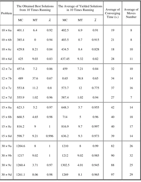
TABLE 5. The Obtained Results of Ts Algorithm for Medium and Large-Sized Instances.

Problem

The Obtained Best Solutions from 10 Times Running

MC MT

λ

The Average of Yielded Solutions in 10 Times Running

MC MT λ

Average of Converging Time (s.)

Average of Moves Number

10 × 6 a 401.1 6.4 0.92 402.5 6.9 0.91 19 8

10 × 6 b 385.4 0 0.94 403.5 0.7 0.915 21 8

10 × 6 c 429.8 8.21 0.84 434.5 8.4 0.828 18 10

10 × 6 d 425 9.03 0.83 437.45 9.32 0.82 28 11

12 × 7 a 457.6 7.2 0.86 459 7.21 0.84 32 10

12 × 7 b 489 37.6 0.67 0.65 38.8 0.65 34 14

12 × 7 c 553.8 11.2 0.8 573.7 12 0.775 37 16

12 × 7 d 555.9 1.02 0.96 587.4 1.02 0.94 27 7

15 × 8 a 623.3 5.2 0.97 648.3 5.7 0.955 42 14

15 × 8 b 668.5 4.65 0.98 714 5 0.96 40 18

15 × 8 c 816.2 9 1 816.9 9.7 0.997 40 17

15 × 8 d 598.7 9.21 0.996 636.2 9.3 0.973 39 14

30 × 9 a 1204.6 8 1 1210 8 0.99 82 26

30 × 9 b 1217 9.02 1 1212 9.02 0.985 90 32

30 × 9 c 1260.4 3.71 0.97 1302.5 4.01 0.945 88 25

9. REFERENCES

1. Khuri, S. and Miryala, S.R., “Genetic Algorithms for Solving Open Shop Scheduling Problems, in: Barahona, P. and Alferes, J.J. (Eds.)”, Lecture Notes in Artificial Intelligence, Springer-Verlag, Berlin, Germany, Vol. 1695, (1999) 357-368.

2. Low, C. _{and Yeh, Y., “Genetic Algorithm-Based}

Heuristics for an Open Shop Scheduling Problem with Setup, Processing, and Removal Times Separated”,

Robotics and Computer-Integrated Manufacturing, Vol. 25, (2009), 314-322.

3. Brucker, P., Johann, H., Bernd, J. and Birgit, W., “A Branch and Bound Algorithm for the Open Shop Problem”, Discrete Applied Mathematics, Vol. 76, (1997), 43-59.

4. Liaw, C., “An Iterative Improvement Approach for the Non Preemptive Open Shop Scheduling Problem”,

European Journal of Operational Research, Vol. 111, (1999), 509-517.

5. Tavakkoli-Moghaddam, R., Taheri, F. and Bazzazi, M., Multi-Objective Uunrelated Parallel Machines Scheduling with Sequence-Dependent Setup Times and Precedence Constraints, International Journal of Engineering, Transaction A: Basic, Vol. 21, (2008), 269-278.

6. T’kindt, V., Monmarche, N., Tercinet, F., Laugt, D., “An Ant Colony Optimization Algorithm to Solve 2 2-Machine Bi-Criteria Flow Shop Scheduling Problem”,

European Journal of Operational Research, Vol. 142, (2002), 250-257.

7. Liaw, C., “Applying Simulated Annealing to the Open Shop Scheduling Problem”, IIE Transactions, Vol. 31, (1999), 457-465.

8. Liaw, C., “A Tabu Search Algorithm for the Open Shop Scheduling Problem”, Computers and Operations Research, Vol. 26, (1999), 109-126.

9. Liaw, C., “An Efficient Tabu Search Approach for the Two-Machine Preemptive Open Shop Scheduling Problem”, Computers and Operations Research, Vol. 30, (2003), 2081-2095.

10. Bertel, S. and Billaut, J., “A Genetic Algorithm for an Industrial Multiprocessor Fow Shop Scheduling Problem with Recirculation”, European Journal of Operational Research, Vol. 159, (2004), 651-662. 11. Tavakkoli-Moghaddam,R.and Mehdizadeh,E.,“ANew

ILP Model for Identical Parallel-Machine Scheduling with Family Setup Times Minimizing the Total Weighted Flow Time by a Genetic Algorithm”,

International Journal of Engineering, Transaction A: Basic, Vol. 20, (2007), 183-194.

12. Cheng, R., Gen, M. and Tsujimura, Y., “Tutorial Survey of Job Shop Scheduling Problems using Genetic Algorithms, Part II: Hybrid Genetic Search Strategies”,

Computers and Industrial Engineering, Vol. 36, (1999), 343-364.

13. Zhou, H., Feng, Y. and Han, L., “The Hybrid Heuristic Genetic Algorithm for Job Shop Scheduling”,

Computers and Industrial Engineering, Vol. 40, (2001), 191-200.

14. Park, B.J., Choi, H.R. and Kim, H.S., “Hybrid Genetic Algorithm for the Job Shop Scheduling Problems”,

Computers and Industrial Engineering, Vol. 45, (2003), 597-613.

15. Goncalves, J.F. and De Magalha es Mendes, J.J., “A Hybrid Genetic Algorithm for the Job Shop Scheduling Problem”, European Journal of Operational Research, Vol. 167, (2005), 77-95.

1 2 3 4 5 6 7 8

0.87 0.875 0.88 0.885 0.89 0.895 0.9 0.905 0.91

T

h

e

L

H

A

g

g

re

g

a

ti

o

n

F

u

n

c

ti

o

n

V

a

lu

e

Neighborhood Search

16. Tseng, L.Y. and Lin, Y.T., “A Hybrid Genetic Algorithm for the Flow Shop Scheduling Problem”,

Lecture Notes in Artificial Intelligence, Vol. 4031, (2006), 218-227.

17. Liaw, C., “A Hybrid Genetic Algorithm for the Open Shop Scheduling Problem”, European Journal of Operational Research, Vol. 124, (2000), 28-42. 18. Sule, D.R., “Industrial Scheduling”, PWS Publishing

Company, Boston, U.S.A., (1997).

19. Torabi, S. A., Hassini, E., “An Interactive Possibilistic Programming Approach for Multiple Objective Supply Chain Master Planning”, Fuzzy Sets and Systems, Vol. 159, (2008), 193-214.

20. Zimmermann, H.J., “Fuzzy Programming and Linear Programming with Several Objective Functions”, Fuzzy Sets and Systems, Vol. 1, (1978), 45-55.

21. Lai, Y.J. and Hwang, C.L., “Possibilistic Linear Programming for Managing Interest Rate Risk”, Fuzzy Sets and Systems, Vol. 54, (1993), 135-146.

22. Lai, Y.J. and Hwang, C.L., “Fuzzy Multiple Objective Decision Making Methods and Applications”, Springer-Verlag, Berlin, Germany, (1994).

23. Werners, B., “Aggregation Models in Mathematical Programming, in: Mitra, G., Greenberg, H.J., Lootsma, F.A., Rijckaert, M.J., Zimmermann, H.-J. (Eds.), “Mathematical Models for Decision Support”, Springer-Verlag, Berlin, Germany, (1988), 295-305.

24. Selim, H. and Ozkarahan, I., “A Supply Chain Distribution Network Design Model: An Interactive Fuzzy Goal Programming-Based Solution Approach”,

International J. of Advanced Manufacturing Technology, Vol. 36, (2008), 401-418.

25. Li, X.Q., Zhang, B. and Li, H., “Computing Efficient Solutions to Fuzzy Multiple Objective Linear Programming Problems”, Fuzzy Sets and Systems, Vol. 157, (2006), 1328-1332.

26. Glover, F., “Tabu Search-Part I”, ORSA Journal on Computing, Vol. 1, (1989), 190-206.

27. Glover, F., “Tabu Search-Part II”, ORSA Journal on Computing, Vol. 2, (1990), 4-32.