Hermite Wavelet Collocation Method for the Numerical Solution of Integral and Integro - Differential Equations

(1)

ISSN: 2231-5373

http://www.ijmttjournal.org

Page 215

Hermite Wavelet Collocation Method for the

Numerical Solution of Integral and

Integro-Differential Equations

Ravikiran A. Mundewadi

#1

, Bhaskar A. Mundewadi

*2

#

P. A. College of Engineering, Mangalore, Karnataka, India. *_{Govt. First Grade College for Women’s, Bagalkot, Karnataka, India.}

Abstract — Hermite wavelet collocation method for the numerical solution of Volterra, Fredholm, mixed Volterra-Fredholm integral equations, integro-differential equations and Abel’s integral equations. The method is based upon Hermite polynomials and Hermite wavelet approximations. The properties of Hermite wavelet is first presented and the resulting Hermite wavelet matrices are utilized to reduce the integral and integro-differential equations into system of algebraic equations to get the required Hermite coefficients are computed using Matlab. This technique is tested, some numerical examples and compared with the exact and existing method. Error analysis is worked out, which shows the efficiency of the proposed method.

Keywords — Hermite wavelet, Collocation method, Integral equations, Integro-differential equations.

AMS Classification code: 65R20, 45B05, 45D05, 45J05, 45E10.

I. INTRODUCTION

Wavelets have found their way into many different fields of science and engineering. Wavelets theory is a pretty new and a budding tool in applied mathematical research area. It has been applied in a broad range of engineering disciplines; particularly, signal analysis for waveform representation and segmentations, time-frequency analysis and quick algorithms for easy implementation. Wavelets permit the accurate representation of a variety of functions and operators. Moreover, wavelets establish a connection with quick numerical algorithms [1, 2]. Since from 1991 the various types of wavelet method have been applied for the numerical solution of different kinds of integral equations, a detailed survey on these papers can be found in [3].

Integral and integro-differential equation is one of the important topics in applied mathematics and also found its applications in various fields of science and engineering. There are several numerical methods for approximating the solution of integral and integro-differential equations is known and many different basic functions have been used. Application of different wavelets has been introduced for solving integral and integro-differential equations. For solving these equations, such as Lepik and tamme [4-10] applied the Haar wavelet method. Maleknejad has introduced rationalized haar wavelets [11, 12], Legendre wavelets [13], Hermite Cubic spline wavelet [14], and Coifman wavelet [15]. Babolian and Fattahzadeh [16] have applied chebyshev wavelet operational matrix of integration. Galerkin methods for the constructions of orthonormal wavelet bases approach by Liang et al. [17]. Yousefi and Banifatemi [18] have introduced a new CAS wavelet. Gao and Jiang [19], proposed the trigonometric Hermite wavelet approximation for solving integral equations of second kind with weakly singular kernel. Abdalrehman [20] has solved an algorithm for nth order integro-differential equations by using Hermite Wavelets Functions. Ali et al. [21], have introduced the Hermite Wavelet Method for Boundary Value Problems, Saeed and Rehman [22], applied the Hermite Wavelet Method for Fractional Delay Differential Equations. Ramane et al. [31] have applied a new Hosoya polynomial of path graphs for the numerical solution of Fredholm integral equations. In this paper, we proposed the Hermite wavelet (HW) collocation method for the numerical solution of integral and integro-differential equations. The proposed method is explained and demonstrated the efficiency of the scheme than the others existing method by presenting some of the illustrative examples.

II. Properties of Hermite Wavelets

2.1 Wavelets

(2)

ISSN: 2231-5373

http://www.ijmttjournal.org

Page 216

1

2

,

( )

,

0

a b

t

b

t

a

a b

R

a











_





_









(2.1)

If we restrict the parameters a and b to discrete values as aa₀k,b p b a₀ ₀k,a₀1,b₀0 and p, and k

positive integer, from Eq. (2.1) we have the following family of discrete wavelets: 1

2

,

( )

(

0 0

)

k

k p

t

a

a t

pb











where

, ( ) k p t



form wavelet basis for

L R

2

( )

. In particular, when

a

₀



2

and 0

1 b



, then



_{k p}_, ( )t forms an orthonormal basis.

2.2 Hermite wavelet

Hermite wavelet

H

_{p q}_,

( )

t



H k n q t

( , , , )

ˆ

has four arguments;

k



2,3,...,

n

ˆ



2 p



1,

1

1, 2,3,..., 2

k

,

p





q

is the order of the Hermite polynomials and

t

_{is the normalized time. They are defined} on the interval [0, 1) by:

/ 2 ˆ 1 ˆ 1 2 2 ,

1 _ˆ

2 (2

),

,

( )

₂

0,

.

k k

k k n n

q p q

q

h

t

n

t

H

t

otherwise

 







 



 





(2.2)

where

q



0,1, 2,...,

M



1,

p



1, 2,3,..., 2

k1. The coefficient

1

2 q



is for orthonormality, the dilation parameter is

_a



2

k_{and translation parameter is}

_b



_n

_ˆ2

k_.

Here,h t_q( )is the well-known Hermite polynomial of order q, which are orthogonal with respect to the weight function

w t

( )



e

t2 in the interval

[

 

, ]

and satisfy the following recursive formula [22],

0

( )

1,

1

( )

2 h t



h t



t

1

( )

2 ( )

2

1

( ),

1, 2,3,....

m m m

h

_

t



th t



mh

_

t

m



The six basis functions are given by:









10 11

2 12

20 21

2 22

( )

2

1 ( )

2 6 (4

1)

; 0

,

2 ( )

10 4(4

1)

2 ( )

2

1 ( )

2 6 (4

3)

;

1

2 ( )

10 4(4

3)

2 H

t

H

t

H

t

H

t

H

t

H

t











_

 







_

_











_

 







_

_

For k = 2 implies q = 1, 2 and M=3 implies p = 0, 1, 2 then using collocation points

0.5 ,

1, 2,

,

j

N

t

N







,Eq. (2.2) gives the Hermite wavelet matrix of order

(

N



2

k1

M

)

6x6 as,

6 6

1.4142 1.4142 1.4142 0 0 0

-3.2660 0

3.2660 0 0 0

-0.7027 -6.3246 -0.7027 0 0

( )

H t

_



0

0 1.4142 1.4142 1.4142

0

0 -3.2660 0 3.2660

0

0 -0.7027 -6.3246 -0.7027













(3)

ISSN: 2231-5373

http://www.ijmttjournal.org

Page 217

8 8

1.4142 1.4142 1.4142 1.4142 0 0 0 0

-3.6742 -1.2247 1.2247 3.6742 0 0 0

( )

H t





0 0.7906 -5.5340 -5.5340 0.7906 0 0 0 0

21.0468 10.7573 -10.7573 -21.0468 0 0 0 0

0 0 0 0 1.4142 1.4142 1.4142 1.4142

0 0 0 0 -3.6742 -1.2247 1.2247 3.6742

0 0 0 0 0.7906 -5.5340 -5.5340 0.7906

0 0 0 0 21.0468 10.7573 -10.7573 -21.0468





















































III. Hermite Wavelet Collocation Method of Solution

In this section, we present a Hermite wavelet (HW) collocation method for solving integral and integro-differential equations.

3.1 Integral Equations

Fredholm Integral equations:

Consider the Fredholm integral equations,

1 1 0

( )

( , ) ( )

,

u t



f t





k t s u s ds

(3.1)

where

f t

( )



L

2

[0,1),

k t s

₁

( , )



L

2

([0,1) [0,1))



and

u t

( )

is an unknown function.

Let us approximate

f t

( )

,

u t

( )

, and

k t s

₁

( , )

by using the collocation points

t

_i as given in the above section 2.2. Then the numerical procedure as follows:

STEP 1: Let us first approximate

f t

( )



X

T



( ),

t

and

u t

( )



Y

T



( ),

t

(3.2) Let the function

f t

( )



L

2

[0,1]

may be expanded as:

, , 1 0

( )

n m n m

( ),

n m

f t

x

H

t

 

 





(3.3)

where

x

n m,



( ( ),

f t H

n m,

( )).

t

(3.4) In (3.4), (. , .) denotes the inner product.

If the infinite series in (3.3) is truncated, then (3.3) can be rewritten as:

1

2 1

, , 1 0

( )

( ),

k

M

T n m n m

n m

f t

x

H

t

X

t

 _

 









(3.5)

where X and



( )

t

are N1matrices given by:

1 1

1

10 11 1, 1 20 2, 1 2 ,0 2 , 1 1 2 2

[

,

,...,

,

,...,

]

[ ,

,...,

] ,

k k

k

T

M M M

T M

X

x

x x

x

 



  



(3.6)

and

1 1

1

10 11 1, 1 20 2, 1 ₂ _,0 ₂ _, ₁ 1 2 2

( ) [

( ),

( ),...,

( ),

( ),...,

( )]

[

( ),

( ),...,

( )] .

k k

k

T

M M _M

T M

t

H

t H t

H

t H

t

H

t

H

t

H

t

H t H t

H

t

 



  

 



(3.7)

STEP 2: Next, approximate the kernel function as:

k t s

₁

( , )



L

2

([0,1] [0,1])



1( , ) ( ) 1 ( ),

T

k t s  t K s (3.8)

(4)

ISSN: 2231-5373

http://www.ijmttjournal.org

Page 218

[

K

1

]

ij



(

H t

i

( ), ( ( , ),

k t s H s

1 j

( ))).

i.e., _(3.9)

STEP 3: Substituting Eq. (3.2) and Eq. (3.8)in Eq. (3.1), we have:





1

1 0

1 1 ₀

1

( )

( )(

),

T T T T

T T

t Y

t X

t K

s

s Yds

t Y

t X

t K

s

s ds Y

t Y

t

X

K Y



 

 



 

 



 





Then we get a system of equations as,

1

(

I



K Y

)



X

,

where,

1

0

( )

T

I

  



s

s ds

is the identity matrix. (3.10) By solving this system obtain the vector Hermite wavelet coefficients ‘Y’ and substituting in step 4.

STEP 4:

u t

( )



Y

T



( )

t

This is the required approximate solution of Eq. (3.1).

Volterra Integral equations:

Consider the Volterra integral equations with convolution but non-symmetrical kernel

2 0

( )

( , ) ( )

,

[0,1]

t

u t



f t





k t s u s ds

t



(3.11)

where

f t

( )



L

2

[0,1),

k t s

₂

( , )



L

2

([0,1) [0,1))



and

u t

( )

Let us approximate

f t

( )

,

u t

( )

, and

k t s

₂

( , )

by using the collocation points

t

_i as given in the above section 2.2. Then the numerical procedure as follows:

STEP 1: The Eq. (3.11) can be rewritten in Fredholm integral equations, with a modified kernel

k t s



2

( , )

and

solved in Fredholm form [23] as,

2 0

( )

( , ) ( )

,

t

u t



f t





k t s u s ds



(3.12)

where,

2 2

( , ),

0 ( , )

0,

1. k t s

s t

k t s

t s

 



 

_{ }





STEP 2: Let us first approximate

f t

( )

and

u t

( )

as given in Eq. (3.2),

STEP 3: Next, we approximate the kernel function as:

k t s



₂

( , )



L

2

([0,1] [0,1])



2

( , )

( )

2

( ),

T

k t s







t



K



s

(3.13)

where

K

₂ is

2

k1

M



2

k1

M

_{matrix, with}

2 2

(

K

)

_ij



(

H t

_i

( ), ( ( , ),

k t s H s



_j

( ))).

i.e.,

K

₂



_





T

( )

t

_



1





_

k t s



₂

( , )



_

 



( )

s



1 _(3.14)

STEP 4: Substituting Eq. (3.2) and Eq. (3.13)in Eq. (3.12), we have:





1

2 0

1 2 ₀

2

( )

( )(

),

T T T T

T T

t Y

t X

t K

s

s Yds

t Y

t X

t K

s

s ds Y

t Y

t

X

K Y



 

 



 

 



 





Then we get a system of equations as,



 



1 1

1

( )

1

( , )

( )

T

(5)

ISSN: 2231-5373

http://www.ijmttjournal.org

Page 219

2

(

I



K Y

)



X

,

where,

1

0

( )

,

T

I

  



s

s ds

is the identity matrix. (3.15) By solving this system obtain the vector Hermite wavelet coefficients ‘Y’ and substituting in step 5.

STEP 5:

u t

( )



Y

T



( )

t

Fredholm-Volterra integral equations:

Consider the Fredholm-Volterra integral equation of the second kind, 1

1 2

0 0

( )

( , ) ( )

,

x

u t



f t





k t s u s ds





k t s u s ds

(3.16)

where 2 2

1 2

( ) [0,1), ( , ) and ( , ) ([0,1) [0,1))

f t L k t s k t s L  are known function and

u t

( )

Let us approximate

f t

( )

,

u t

( )

,

k t s

₁

( , ) and

k t s

₂

( , )

by using collocation points as follows: STEP 1: Let us first approximate

f t

( )

and

u t

( )

as given in Eq. (3.2),

STEP 2: Substituting Eq. (3.2), Eq. (3.9) and Eq. (3.14) in Eq. (3.16), we get a system of N equations with N

unknowns,

i.e.,

(

I



K

₁



K Y

₂

)



X

.

(3.17) where, I is an identity matrix.

By solving this system we obtain the Hermite wavelet coefficient ‘Y’ and then substitute in step 3.

STEP 3:

_{u t}

( )

_

_Y

T



( )

_t

Abel integral equations:

Consider the Abel integral equation, First kind:

0

( )

, 0

1, 0

1,

(

)

t

u s

f t

ds

t

s





 

 





(3.18)

Second kind:

0

( )

, 0

1

t

u s

u t

f t

ds

t s

t

s











(3.19)

Numerical procedure as follows:

STEP 1: We first approximate u(t) as truncated series defined in Eq. (3.5). That is,

( )

T

( )

u t

 

Y

t

(3.20)

where Y and



( )

t

are defined similarly to Eqs. (3.6) and (3.7). STEP 2: Then substituting Eq. (3.20) in Eqs. (3.18) and (3.19), we get

First kind:

0

( )

,

(

)

t T

Y

s

f t

ds

t

s











(3.21)

Second kind:

0

( )

, 0

1

t T

T

Y

s

Y

t

f t

ds

t s

t

s













(3.22)

STEP 3: Substituting the collocation point

t

_i in Eqs. (3.21) and (3.22), we obtain, First kind:

0

( )

(

)

i t T

i

Y

s

f t

ds

t

s











(3.23)

1 1

0

( )

, where

(

)

i t _T T

i

Y

s

f t

Y G

G

ds

t

s











Second kind:

0

( )

,

i t T T

i i

i

Y

s

Y

t

f t

ds

t

s









(6)

ISSN: 2231-5373

http://www.ijmttjournal.org

Page 220

2 2

0

( )

( ( )

)

, where

t T T

i

Y

s

Y

t

G

f

G

ds

t

s











STEP 4: Now, we get the system of algebraic equations with unknown coefficients. First kind:

f



Y G

T ₁

Second kind:

Y K

T



f

, where

K

 

( ( )

t

_i



G

₂

)

STEP 5: By solving the above system of equations, we obtain the Hermite wavelet coefficients ‘Y’ and then

substitute in Eq. (3.20), we obtain the approximate solution of Eq. (3.18) and Eq. (3.19).

3.2 Integro-differential Equations

Fredholm Integro-differential equations:

In this section, we concerned about a technique that will reduce Fredholm integro-differential equation to an equivalent Fredholm integral equation. This can be easily done by integrating both sides of the integro-differential equation as many times as the order of the derivative involved in the equation from 0 to t for every time we integrate, and using the given initial conditions. It is worth noting that this method is applicable only if the Fredholm integro-differential equation involves the unknown function u(t) only, and not any of its derivatives, under the integral sign [24].

Consider the Fredholm integro-differential equations,

1

( ) ( )

1 0

( )

( , ) ( )

,

n l

l

u

t



f t





k t s u s ds u



b

(3.25)

where

f t

( )



L

2

[0,1),

k t s

₁

( , )



L

2

([0,1) [0,1))



and

u

( )n

( )

t

Where

u

( )n

( )

t

is the nthderivative of

u t

( )

w. r. t t and

b

_l are constants that define the initial conditions. Let us first, we convert the Fredholm integro-differential equation into Fredholm integral equation, then we reduce it into a system of algebraic equations as given in Eq. (3.10), using this system we solve the Eq. (3.25). Then we obtain the approximate solution of equation.

Volterra Integro-differential equations:

In this section, we concerned with converting to Volterra integral equations. We can easily convert the Volterra integro-differential equation to equivalent Volterra integral equation, provided the kernel is a difference kernel defined by k(t, s) = k(t − s). This can be easily done by integrating both sides of the equation and using the initial conditions. To perform the conversion to a regular Volterra integral equation, we should use the well-known formula, which converts multiple integrals into a single integral [24].

i.e.,

1

0 0 0 0

1 ...

( )

(

)

( )

(

1)!

t t t t

n n

u t dt

t

s

u s ds

n











Consider the Volterra integro-differential equations,

( ) ( )

2 0

( )

( , ) ( )

,

t

n l

l

u

t



f t





k t s u s ds u



b

(3.26)

where 2 2

2

( ) [0,1), ( , ) ([0,1) [0,1))

f t L k t s L  and

u

( )n

( )

t

where

u

( )n

( )

t

is the nth derivative of

u t

( )

with respect to t and

b

_l are constants that define the initial conditions.

Let us first, we convert the Volterra integro-differential equation into Volterra integral equation, then we reduce it into a system of algebraic equations as given in Eq. (3.15), using this system we solve the Eq. (3.26). Then we obtain the approximate solution of equation.

IV. Convergence Analysis Theorem: The series solution _, _,

1 0

( )

_{p q} _{p q}

( )

p q

u t



 

_ _

x

H

t

defined in Eq. (3.5) using Hermite wavelet collocation method converges to

u t

( )

as given in [25].

Proof: Let

L R

2

( )

be the Hilbert space and H_{p q}_, defined in Eq. (3.2) forms an orthonormal basis. Let

1 , , 0

( )

M _{p i} _{p i}

( )

i

(7)

ISSN: 2231-5373

http://www.ijmttjournal.org

Page 221

Let us denote

,( ) ( ) p i

H t H t and let



_j



u t H t

( ), ( ) .

Now we define the sequence of partial sums S_pof (



_jH t( ));_j Let S_p and S_qbe the partial sums with

.

p



q

we have to prove S_p is a Cauchy sequence in Hilbert space. Let

1

( ).

p

p _i j j

S





_



H t

Now 2

1 1

( ),

( )

.

p p

p j j j

i j

u t S

u t



H t



 









we claim that

2 2

1

,

.

p

p q j

j q

S



p

q

 









Now

2

1 1 1 1

( )

( ),

( )

,

.

p p p p

j j j j j j j

j q j q j q j q

H t

for p

q



       







Therefore, 2 2 1 1

( )

,

.

p p

j j j

j q j

H t

for p

q



  







From Bessel’s inequality, we have 2

1 p

j j





is convergent and hence

2

1

( )

0 ,

p

j j

j q

H t

as q p



 



 



So, 1

( )

0

p j j j q

H t



 





and {S_p} is a Cauchy sequence and it converges to s (say). We assert that

u t

( )



s

Now

( ),

( )

_j

,

( )

_j

( ),

( )

_j

lim

_p

,

( )

_j _j _j _j

p

s

u t H t

s H t

u t H t

S

H t



















, This implies,

( ),

( )

_j

0 s u t H t





Hence

u t

( )



s

and

1

( )

p

j j

i



H t



converges to

u t

( )

as

p

 

and proved.

V. Numerical experiments

In this section, we present Hermite wavelet (HW) collocation method for the numerical solution of integral and integro-differential equations in comparison with existing method to demonstrate the capability of the present method and error analysis are shown in tables and figures. Error function is presented to verify the accuracy and efficiency of the following numerical results:





2 max

1

( )

n

e i a i e i a i

i

E

Error function

u t

_

u t











where,𝑢_𝑒 and𝑢_𝑎 are the exact and approximate solution respectively.

Example 5.1 Let us consider the linear Fredholm integral equation [12],

1 1 0

1 ( )

( )

1

t

e

ts

u t

e

e u s ds

t



_

 





, 0 t 1 (5.1)

which has the exact solution

u t

( )



exp( )

t

. Where

1

1 ( )

1

t t

e

f t

e

t



_

 



and kernel 1

( , )

ts

(8)

ISSN: 2231-5373

http://www.ijmttjournal.org

Page 222

Next, approximate the kernel function as: 2

1( , ) ([0,1] [0,1])

k t s L 

1( , ) ( ) 1 ( ), T

k t s  t K s

where

K

₁ is 1 1

2k M2k M matrix, with [K₁]ij (H ti( ), ( ( , ),k t s H₁ j( ))).s



 



1 1

1

( )

1

( , )

( )

T

K





_



t



_





k t s

 

s



Next, substituting the function

f t

( )

,

u t

( )

, and

k t s

₁

( , )

in Eq. (5.1), then using the collocation points

t

_i, we get the system of algebraic equations with unknown coefficients for k = 2 and M = 4 (N = 8), as an order

8 8



as follows:





1

1 0

1 1

0 1

( )

( )(

),

T T T T

T T

t Y

t X

t K

s

s Yds

t Y

t X

t K

s

s ds Y

t Y

t X

K Y



 

 



 

 



 





1

(

I



K Y

)



X

,

where,

1

0

( )

T

I

  



s

s ds

is the identity matrix. We get, X = [-0.4963 0.0048 0.0010 0.0001 -0.4152 0.0203 0.0020 0.0001],

1

0.5336 0.0099 0.0002 0.0000 0.6094 0.0120 0.0002 0.0000

0.0099 0.0030 0.0001 0.0000 0.0334 0.0038 0.0001 0.0000

0.0002 0.0001 0.0000 0.0

K



000 0.0013 0.0003 0.0000 0.0000

0.0000 0.0000 0.0000 0.0000 0.0000 0.0000 0.0000 0.0000

0.6094 0.0334 0.0013 0.0000 0.8940 0.0499 0.0019 0.0001

0.0120 0.0038 0.0003 0.0000 0.0499 0.0074 0.0005 0.0000

0.0002 0.0001 0.0000 0.0000 0.0019 0.0005 0.0000 0.0000

0.0000 0.0000 0.0000 0.0000 0.0001 0.0000 0.0000 0.0000





















































By solving this system of equations, we obtain the Hermite wavelet coefficients,

Y = [0.9343 0.0656 0.0032 0.0001 1.5261 0.1088 0.0053 0.0002]

and substituting these coefficients in

u t

( )



Y

T



( ),

t

we get the approximate solution

u t

( )

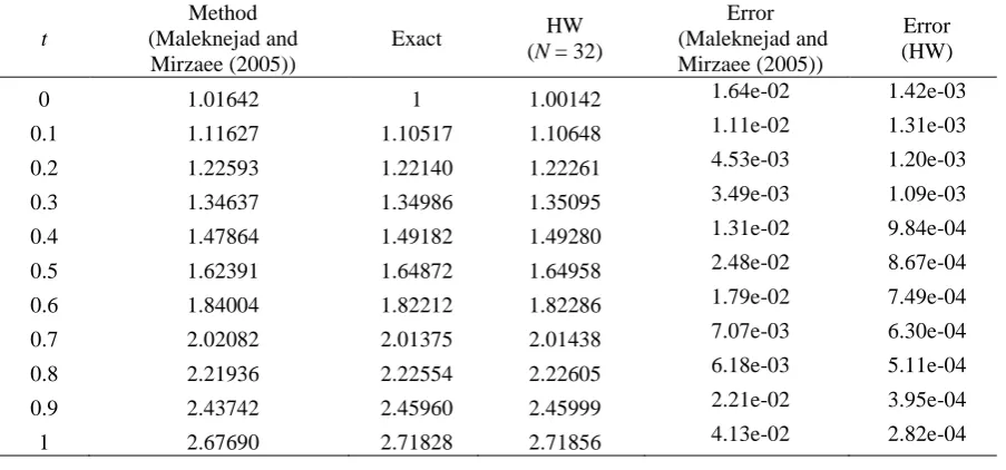
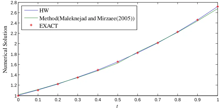
, which is compared with existing method (Haar wavelet) and exact solutions are shown in table 1. Graphically presented in figure 1 in comparison of numerical solutions with exact solutions and existing method.

Table 1 Numerical results of the example 5.1.

t

Method (Maleknejad and Mirzaee (2005))

Exact HW (N = 32)

Error (Maleknejad and

Mirzaee (2005))

Error (HW)

0 1.01642 1 1.00142 1.64e-02 1.42e-03

(9)

ISSN: 2231-5373

http://www.ijmttjournal.org

Page 223

Fig. 1 Comparison of HW solution with exact solution and existing method.

Example 5.2 Next, consider [12]

1

0

( )

( , ) ( )

u t

 

t



k t s u s ds

,

0  

t

1

(5.2)

where,

( , )

,

.

t

s

k t s

s

t





 

_



u t

( ) sec(1) sin( ).





t

We apply the Hermite wavelet approach and solved Eq. (5.2) yields the approximate values of 𝑢(𝑡)with the help of Hermite wavelet coefficient ‘Y ’ for k = 2, M = 4 (N

= 8) as an order

8 8



as follows,

X = [0.1768 0.0510 0 0.0000 0.5303 0.0510 0.0000 0],

1

0.0786 0.0180 -0.0009 0.0000 0.1250 0.0000 0 0

0.0180 0.0558 -0.0000 0.0085 0.0361 0.0000 0 0

0.0009 0.0000 0.0016

-K



0.0000 0 0 0 0

0.0000 0.0085 0.0000 0.0015 0.0000 0.0000 0 0.0000

0.1250 0.0361 0 0.0000 0.3286 0.0180 -0.0009 0.0000

0.0000 -0.0000 -0.0000 -0.0000 0.0180 0.0558 0.0000 0.0085

0 0 0 0 -0.0009 0.0000 0.0016 -0.0000

0.0000 0.0000 0.0000 0.0000 -0.0000 0.0085 -0.0000 0.0015





















































Y = [0.3096 0.0926 -0.0003 0.0008 0.8544 0.0704 -0.0007 0.0006]. Then substituting these coefficients in

u t

( )



Y

T



( )

t

, we obtain the approximate solutions and compared with existing method (Haar wavelet) and exact solutions are shown in table 2 for k = 4 and M = 4 (N = 32). In figure 2, as compared the numerical results with exact solutions and existing method.

t

Method

(Maleknejad and Mirzaee (2005))

Exact HW (N = 32)

Error (Maleknejad and Mirzaee (2005))

Error (HW)

0 0.02892 0 0.00319 2.89e-02 3.19e-03

0.1 0.20205 0.18477 0.18138 1.72e-02 3.38e-03 0.2 0.37341 0.36770 0.36639 5.71e-03 1.30e-03 0.3 0.54148 0.54695 0.54555 5.47e-03 1.40e-03 0.4 0.70480 0.72074 0.71933 1.59e-02 1.40e-03

0 0.1 0.2 0.3 0.4 0.5 0.6 0.7 0.8 0.9 1

1 1.2 1.4 1.6 1.8 2 2.2 2.4 2.6 2.8

t

N

u

m

e

ri

c

a

l

S

o

lu

ti

o

n

HW

(10)

ISSN: 2231-5373

http://www.ijmttjournal.org

Page 224

0.5 0.86192 0.88733 0.88587 2.54e-02 1.44e-03 0.6 1.05943 1.04505 1.04295 1.43e-02 2.09e-03 0.7 1.19686 1.19233 1.18931 4.53e-03 3.01e-03 0.8 1.32378 1.32769 1.32472 3.91e-03 2.96e-03 0.9 1.43908 1.44979 1.44586 1.07e-02 3.92e-03 1 1.54173 1.55741 1.55269 1.56e-02 4.72e-03

Fig. 2 Comparison of HW solution with exact solution and existing method.

1 0

( )

sin(2

)

cos( ) ( )

u t





t





t u s ds

(5.3)

u t

( )



sin(2



t

)

. We applied the present method and solved Eq. (5.3), we get the approximate values of

u t

( )

with the help of Hermite wavelet coefficients. In table 3, error analysis shows the comparison of Hermite Wavelet with existing method.

1 ₂ ₂

0

( )

sin(2 )

(

) ( )

u t





t





t

  

t

s

s u s ds

(5.4) which has the exact solution

u t

( )



sin(2



t

)

. Solving Eq. (5.4), using the above method, we obtain the approximate values of

u t

( )

with the help of Hermite wavelet coefficients. In table 3, error analysis shows the comparison of Hermite Wavelet with existing method.

1

3 2 2 2

0

( )

2

3 (

) ( )

u t

 

t



t

 

t



t

  

t

s

s u s ds

(5.5) which has the exact

u t

( )

 

2 t

3



3 t

2



t

. Solving Eq. (5.5), we get the approximate solution

u t

( )

with the help of Hermite wavelet coefficients. In table 3, error analysis shows the comparison of Hermite Wavelet with the existing method.

Table 3Comparison of the Error analysis.

N

Example 5.3 Example 5.4 Example 5.5 Method

(Maleknejad and Yousefi (2006b))

(HW)

Max

E

Method (Maleknejad and Yousefi (2006b))

(HW)

Max

E

Method (Maleknejad and Yousefi (2006b))

(HW)

Max

E

4 2.84e-02 6.66e-16 2.84e-02 1.11e-16 1.33e-10 1.38e-17 8 2.38e-03 7.21e-16 2.38e-03 2.22e-16 3.79e-10 6.93e-17 16 2.09e-04 7.77e-16 2.10e-04 7.77e-16 3.26e-10 4.85e-17 32 1.20e-04 8.88e-16 2.00e-04 6.66e-16 4.83e-10 1.24e-16

0 0.1 0.2 0.3 0.4 0.5 0.6 0.7 0.8 0.9 1

0 0.2 0.4 0.6 0.8 1 1.2 1.4 1.6

t

N

u

m

e

ri

c

a

l

S

o

lu

ti

o

n

HW

(11)

ISSN: 2231-5373

http://www.ijmttjournal.org

Page 225

Example 5.6 Let us consider the linear Volterra integral equation [26],

0

1 ( )

( )

,

5

t

u t

 

t



ts u s ds

, 0 t 1 (5.6)

u t

( )



t

exp( /15).

t

3 Where

f t

( )



t

and kernel ₁

( , )

1

5 k t s



ts

.

Firstly, we approximate

f t

( )



X

T



( ),

t

and

u t

( )



Y

T



( ),

t

Next, approximate the kernel function as: 2

2( , ) ([0,1] [0,1])

k t s L 

2( , ) ( ) 2 ( ), T

k t s  t K  s

where

K

₂ is 1 1

2k M2k M matrix, with [K₂]ij (H ti( ), (k t s H₂( , ), j( ))).s



 



1 1

2

( )

2

( , )

( )

T

K





_



t



_





k t s

 

s



Next, substituting the

f t

( )

,

u t

( )

, and

k t s

₂

( , )

in Eq. (5.6) using the collocation point, we get the system of algebraic equations with unknown coefficients for k = 2 and M = 4 (N = 8), as an order

8 8



as follows:





1

2 0

1 2

0 2

( )

( )(

),

T T T T

T T

t Y

t X

t K

s

s Yds

t Y

t X

t K

s

s ds Y

t Y

t X

K Y



 

 



 

 



 





2

(

I



K Y

)



X

,

where,

1

0

( )

T

I

  



s

s ds

is the identity matrix. where, X = [0.1768 0.0510 0 0.0000 0.5303 0.0510 0.0000 0],

2

0.0012 -0.0030 -0.0010 -0.0005 0 0 0 0

0.0007 -0.0105 -0.0006 -0.0018 0 0 0 0

0.0001

K



-0.0013 -0.0002 -0.0002 0 0 0 0

0.0000 -0.0016 -0.0000 -0.0003 0 0 0 0

0.0188 0.0054 0 0.0000 0.0165 -0.0175 -0.0041 -0.0021

0.0018 0.0005 -0.0000 -0.0000 0.0105 -0.0844 0.0005 -0.0140

-0.0000 -0.0000 -0.0000 -0.0000 -0.0010 -0.0062 -0.0015 -0.0012

0.0000 0.0000 0.0000 0.0000 0.0008 -0.0133 0.0004 -0.0023





















































By solving this system of equations, we get the Hermite wavelet coefficients ‘Y’, Y = [0.1768 0.0506 -0.0001 -0.0001 0.5419 0.0526 -0.0008 -0.0003]

and substituting these coefficients in

u t

( )



Y

T



( ),

t

we obtain the approximate solution

u t

( )

as shown in table 4. Maximum error analysis is shown in table 6.

(12)

ISSN: 2231-5373

http://www.ijmttjournal.org

Page 226

Example 5.7 Consider, linear Fredholm integro-differential equations [27],

1

0

'( )

exp( ) exp( )

( )

,

(0)

0,

u t



t



t

 

t



t u s ds

u



0  

t

1

(5.7) which has the exact solution

u t

( )



t

exp( ).

t

Integrating Eq. (5.7) w.r.t t, we get Fredholm integral equation,

1 2

0

( (

2 exp( )))

( )

,

2

2 t t

t

u t

 







u s ds

We applied the Hermite wavelet collocation method and solved the above equation yields the values of

u t

( )

with the help of Hermite wavelet coefficients. Maximum error analysis is shown in table 6.

Example 5.8 Let us consider the linear Volterra integro-differntial equation [28],

0

''( )

1 (

) ( )

,

(0)

1,

'(0)

0,

t

u t

  



t



s u s ds u



u



0 t 1 (5.8) which has the exact solution

u t

( ) cos( ).



t

Integrating Eq. (5.8) twice w.r.t t, we get Volterra integral equation,

2 3

0

1

1 ( )

1 (

)

( )

2

6

t

u t

 

t





t



s

u s ds

We applied the Hermite wavelet collocation method and solved the above equation yields the values of

u t

( )

with the help of Hermite wavelet coefficients. Maximum error analysis is shown in table 6.

Example 5.9 Next, consider the linear Volterra-Fredholm integral equation [24],

1

2 4

0 0

1

1 ( )

(

) ( )

(

) ( )

,

12

4

3

t

u t

 

t

 

t





t



s u s ds





t



s u s ds

0 t 1 (5.9) which has the exact solution

u t

( )



t

2

.

Where

f t

( )



t

and the kernels

k t s

₁

( , )

 

(

t s

)

and

2

( , ) (

)

k t s

 

t s

.

Let us approximate

f t

( )

,

u t

( )

,

k t s

₁

( , ) and

k t s

₂

( , )

as given in Eq. (3.5), Eq. (3.9) and Eq. (3.14) using the collocation points, we get an system of N equations with N unknowns,

i.e.,

(

I



K

₁



K Y

₂

)



X

where, I is an identity matrix, we find, X = [-0.1704 0.0078 0.0048 -0.0000 0.0414 0.0512 0.0035 -0.0001],

1

0.2500 0.0361 0.0000 0.0000 0.5000 0.0361 -0.0000 0.0000 0.0361 0.0000 0.0000 0.0000 0.0361 0.0000 0 0 -0.0000 0.0000 0.0000 0.0000

K 

-0.0000 -0.0000 -0.0000 -0.0000 0.0000 -0.0000 0 -0.0000 0.0000 0.0000 0.0000 0.0000 0.5000 0.0361 -0.0000 0.0000 0.7500 0.0361 0 0.0000 0.0361 0.0000 0 0 0.0361 0.0000 -0.0000 0.0000 -0.0000 -0.0000 -0.0000 -0.0000 0.0000 0.0000 0.0000 0.0000 0.0000 0.0000 0.0000 0.0000 0.0000 0.0000 0.0000 0.0000

 

 

 

2

0.0464 -0.0180 0.0009 -0.0000 0 0 0 0 0.0180 -0.0558 -0.0000 -0.0085 0 0 0 0 0.0009 0

K 

-0.0016 0 0 0 0 0 0.0000 -0.0085 0.0000 -0.0015 0 0 0 0 0.2500 -0.0361 0.0000 -0.0000 0.0464 -0.0180 0.0009 -0.0000 0.0361 -0.0000 0.0000 -0.0000 0.0180 -0.0558 -0.0000 -0.0085 -0.0000 -0.0000 0.0000 -0.0000 0.0009 0 -0.0016 0 0.0000 0.0000 0 0.0000 0.0000 -0.0085 0.0000 -0.0015

 

 

 

By solving this system, we obtain the Hermite wavelet coefficient,

(13)

ISSN: 2231-5373

http://www.ijmttjournal.org

Page 227

Then, substituting in

u t

( )



Y

T



( ),

t

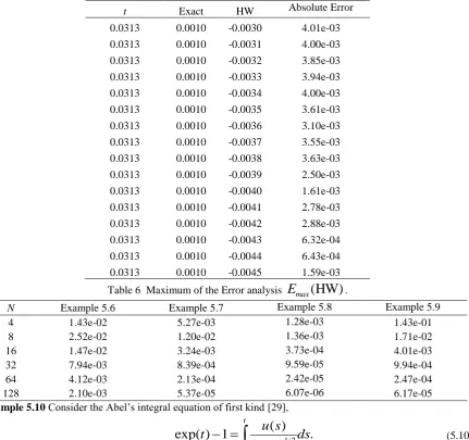
we get the approximate solution of Eq. (5.9) as shown in table 5. Maximum error analysis is shown in table 6.

Table 5 Numerical results of the example 5.2, for N = 16.

t Exact HW Absolute Error 0.0313 0.0010 -0.0030 4.01e-03 0.0313 0.0010 -0.0031 4.00e-03 0.0313 0.0010 -0.0032 3.85e-03 0.0313 0.0010 -0.0033 3.94e-03 0.0313 0.0010 -0.0034 4.00e-03 0.0313 0.0010 -0.0035 3.61e-03 0.0313 0.0010 -0.0036 3.10e-03 0.0313 0.0010 -0.0037 3.55e-03 0.0313 0.0010 -0.0038 3.63e-03 0.0313 0.0010 -0.0039 2.50e-03 0.0313 0.0010 -0.0040 1.61e-03 0.0313 0.0010 -0.0041 2.78e-03 0.0313 0.0010 -0.0042 2.88e-03 0.0313 0.0010 -0.0043 6.32e-04 0.0313 0.0010 -0.0044 6.43e-04 0.0313 0.0010 -0.0045 1.59e-03 Table 6 Maximum of the Error analysis

E

_max

(HW)

.

N Example 5.6 Example 5.7 Example 5.8 Example 5.9 4 1.43e-02 5.27e-03 1.28e-03 1.43e-01 8 2.52e-02 1.20e-02 1.36e-03 1.71e-02 16 1.47e-02 3.24e-03 3.73e-04 4.01e-03 32 7.94e-03 8.39e-04 9.59e-05 9.94e-04 64 4.12e-03 2.13e-04 2.42e-05 2.47e-04 128 2.10e-03 5.37e-05 6.07e-06 6.17e-05

Example 5.10 Consider the Abel’s integral equation of first kind [29],

1/ 2 0

( )

exp( ) 1

.

(

)

t

u s

t

ds

t

s

 





(5.10)

Firstly, consider

u t

( )

 

Y

T

( )

t

(5.11) substituting

u t

( )

in Eq. (5.10), we get

1/ 2 0

( )

exp( ) 1

.

(

)

t T

Y

s

t

ds

t

s



 





(5.12)

Next, we collocate the point

t

_iand substitute in Eq. (5.12),

1/ 2 0

( )

exp( ) 1 .

( )

i

t T i

i

Y s

t ds

t s

  





_(5.13)

Now, we get the system of algebraic equations with unknown coefficients. By solving this system of equations for k = 1 and M = 5 as given,



0.1052 0.3499 0.6487 1.0138 1.4596



f 

1

0.6325 1.0954 1.4142 1.6733 1.8974 -1.8988 -2.2768 -1.6330 -0.3864 1.3145 1.4406 -1.0582 -3.7947 -4.8093 -2.9189 8.5628 14.4390 10.6904 0.6517 -8.7

G 

525 -28.3334 -11.3738 17.7248 23.7824 -5.8776

 

 

(14)

ISSN: 2231-5373

http://www.ijmttjournal.org

Page 228

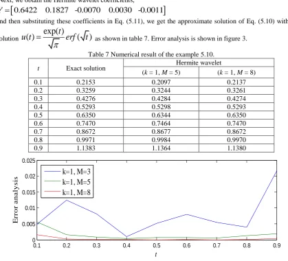
Next, we obtain the Hermite wavelet coefficients,



0.6422 0.1827 -0.0070 0.0030 -0.0011



Y



and then substituting these coefficients in Eq. (5.11), we get the approximate solution of Eq. (5.10) with exact solution

exp( )

( )

t

(

)

u t

erf

t





as shown in table 7. Error analysis is shown in figure 3.

Table 7 Numerical result of the example 5.10.

t Exact solution Hermite wavelet

(k = 1, M = 5) (k = 1, M = 8)

0.1 0.2153 0.2097 0.2137

0.2 0.3259 0.3244 0.3261

0.3 0.4276 0.4284 0.4274

0.4 0.5293 0.5298 0.5293

0.5 0.6350 0.6344 0.6350

0.6 0.7470 0.7464 0.7470

0.7 0.8672 0.8677 0.8672

0.8 0.9971 0.9984 0.9970

0.9 1.1383 1.1364 1.1380

Fig. 3 Error analysis of the example 5.10.

Example 5.11 Next, consider [29],

4/5 0

( )

.

(

)

t

u s

t

ds

t

s







(5.14)

Applying the above method, we obtain the approximate solution

u t

( )

of Eq. (5.14) with the help of Hermite wavelet coefficients. Numerical solution is compared with exact solution

( )

5 sin( )

5 4/5

4 u t

t





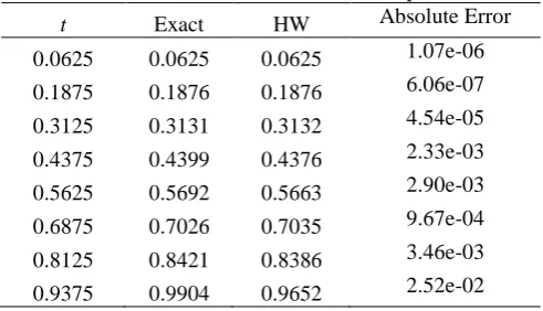
as shown in table 8. Error analysis is shown in figure 4.

t Exact solution Hermite wavelet (k = 1, M = 8)

0.1 0.0371 0.0369

0.2 0.0645 0.0645

0.3 0.0893 0.0893

0.4 0.1124 0.1124

0.5 0.1343 0.1343

0.6 0.1554 0.1554

0.7 0.1758 0.1758

0.8 0.1956 0.1956

0.9 0.2150 0.2149

0.1 0.2 0.3 0.4 0.5 0.6 0.7 0.8 0.9

0 0.005 0.01 0.015 0.02 0.025

t

E

rr

o

r

a

n

a

ly

s

is

(15)

ISSN: 2231-5373

http://www.ijmttjournal.org

Page 229

Fig. 4 Error analysis of the example 5.11.

Example 5.12 Consider the Abel’s integral equation of the second kind [30],

0

4

1 ( )

4 ( )

arcsin

, 0

1.

1

2

1

t

u s

u t

ds

t

s













_

_

 

 











(5.15)

1 ( )

.

1 u t

t





Applying the Hermite Wavelet Collocation Method for solving

Eq. (5.15) with k =1 and M =3, we find,

[4.4785 4.4969 4.4340]

4.8165 5.4142 5.8257

-11.4375 -1.6330 9.9403

-1.1491 -21.6833 -5.9189

f

K











 











Next, we get the Hermite wavelet coefficients,



0.8344 -0.0406 0.0040



Y



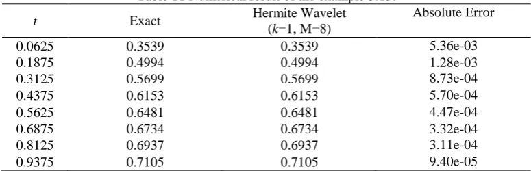
and substituting these coefficients in Eq. (5.11), we get the approximate solution of Eq. (5.15) with exact solution as shown in table 9 and the error analysis is shown in table 10.

t Exact Hermite Wavelet (k=1, M=8)

Absolute Error

0.0625 0.9701 0.9701 1.12e-07

0.1875 0.9177 0.9177 2.47e-08

0.3125 0.8729 0.8729 2.61e-08

0.4375 0.8341 0.8341 1.76e-08

0.5625 0.8000 0.8000 1.68e-08

0.6875 0.7698 0.7698 1.20e-08

0.8125 0.7428 0.7428 1.56e-08

0.9375 0.7184 0.7184 8.33e-09

Table 10 Maximum error analysis of the example 5.12 1

2

k

N





M

Hermite Wavelet

k = 1, M = 3 3.15e-04

k = 1, M = 5 1.17e-05

k = 1, M = 8 1.12e-07

Example 5.13 Lastly, consider [30],

0

( )

2 , 0

1.

t

y s

u t

t

ds

t

s





 





(5.16)

u t

( )

 

1 exp(



t erfc

)

 



t

. We solved the Eq. (5.16) by approaching the present method for k = 1 and M = 5 with the help of Hermite wavelet coefficients, we get the approximate solution as shown in table 11 and the error analysis is shown in table 12.

0.1 0.2 0.3 0.4 0.5 0.6 0.7 0.8 0.9

0 0.5 1 1.5x 10

-3

t

E

rr

o

r

a

n

a

ly

si

s k=1, M=3