Multiclass Boosting: Margins, Codewords, Losses, and Algorithms
Mohammad Saberian [email protected]
Statistical Visual Computing Laboratory, University of California, San Diego La Jolla, CA 92039, USA
Nuno Vasconcelos [email protected]
Statistical Visual Computing Laboratory, University of California, San Diego La Jolla, CA 92039, USA
Editor:Koby Crammer
Abstract
The problem of multiclass boosting is considered. A new formulation is presented, combin-ing multi-dimensional predictors, multi-dimensional real-valued codewords, and proper multiclass margin loss functions. This leads to a number of contributions, such as maximum capacity code-word sets, a family of proper and margin enforcing losses, denoted asγ−φlosses, and two new multiclass boosting algorithms. These are descent procedures on the functional space spanned by a set of weak learners. The first, CD-MCBoost, is a coordinate descent procedure that updates one predictor component at a time. The second, GD-MCBoost, a gradient descent procedure that updates all components jointly. Both MCBoost algorithms are defined with respect to aγ−φ
loss and can reduce to classical boosting procedures (such as AdaBoost and LogitBoost) for binary problems. Beyond the algorithms themselves, the proposed formulation enables a unified treatment of many previous multiclass boosting algorithms. This is used to show that the latter implement different combinations of optimization strategy, codewords, weak learners, and loss function, high-lighting some of their deficiencies. It is shown that no previous method matches the support of MCBoost for real codewords of maximum capacity, a proper margin-enforcing loss function, and any family of multidimensional predictors and weak learners. Experimental results confirm the su-periority of MCBoost, showing that the two proposed MCBoost algorithms outperform comparable prior methods on a number of datasets.
Keywords: Boosting, Multiclass Boosting, Multiclass Classification, Margin Maximization, Loss Function.
1. Introduction
Boosting is a popular approach for classifier design. It is a simple and effective procedure to learn strong decision rules by combination of weak learners. However, most boosting algorithms were designed primarily for binary classification. In many cases, the extension to M-ary problems (of M > 2) is not straightforward. There are many ways to interpret boosting (Schapire and Freund, 2012) and these have been used to justify different multiclass extensions. In this work, we consider the view of boosting as a method for empirical risk minimization, using some optimization proce-dure (usually gradient descent) on the functional space spanned by a set of weak learners (Friedman
c
SABERIAN ANDVASCONCELOS
et al., 1998; Mason et al., 2000). Under this view, the effectiveness of a boosting algorithm is deter-mined by the underlying choices of optimization method, weak learner pool, and risk function. The latter can be further decomposed into a choice of a loss function and an encoding of class labels. All of these are fairly well understood in the binary setting. In some cases, such as the selection of code-word labels, there is virtually universal agreement in the literature, where most algorithms use−1
as the label of “negative” examples and+1for “positives”. On others, there is wide but not univer-sal agreement. For example, while it can be shown that most boosting algorithms implement some form of functional gradient descent (Mason et al., 2000; Zhang, 2004; Buja et al., 2006; Masnadi-Shirazi and Vasconcelos, 2008), there have also been proposals to use second order optimization methods, based on Taylor series expansions (Saberian et al., 2010) and Newton’s method (Fried-man et al., 1998). The remaining aspects are less consensual. Most algorithms differ in terms of the loss function that defines the risk for which they are optimal. Several loss properties, such as encouraging large margins (Vapnik, 1998) and allowing the recovery of class probabilities (Zhang, 2004; Buja et al., 2006; Mease and Wyner, 2008; Masnadi-Shirazi and Vasconcelos, 2008; Reid and Williamson, 2010) have been identified as important, and shown to hold for a large family of functions (Masnadi-Shirazi and Vasconcelos, 2015). Some members of this family, such as the ex-ponential loss of AdaBoost (Freund and Schapire, 1997), the logit loss of LogitBoost (Friedman et al., 1998), the hinge loss of support vector machines (Vapnik, 1998) or the Savage loss of Sav-ageBoost (Masnadi-Shirazi and Vasconcelos, 2008), have been widely used in practice. Finally, weak learners tend to vary with the application. Popular choices include weak classifiers, such as the decision stumps or shallow decision trees commonly used in computer vision (Viola and Jones, 2004; Dollar et al., 2012), and regression models (Friedman et al., 1998).
To date, there have been no comprehensive efforts to extend this understanding to the M-ary case. While boosting components such as the optimization strategy generalize in a straightforward manner, others do not. In particular, many label encodings and loss functions are possible. There is limited understanding of what constitutes a good encoding or when a loss function is proper (allows the recovery of class conditional probabilities). As we will see later on, some popular choices for these components are quite suboptimal. In fact, for multiclass boosting, it is not even easy to guaran-tee that a set of multiclass weak learners can be boosted. For binary classification, it is well known this is possible as long as a weak learner with “less than50%error” can be found in all bosting iter-ations. Since this only requires a weak learner marginaly better than random guessing, the condition can be met trivially. However, forM-ary classification, the accuracy of a random classifier is only
100
M %. In this case, straightforward extensions of binary boosting algorithms that require multiclass
In this work, we study multiclass boosting with the goal of an integrated understanding of the roles of the optimization strategy, label codewords, weak learners, and multiclass risk. This leads to a new formulation of the problem based on 1) multi-dimensional predictors, 2) multi-dimensional real valued codewords, and 3) proper multiclass margin loss functions. We start by studying the role of the label encoding, showing that the selected codewords impose an upper bound on the max-imum margin achievable by any predictor. This is denoted the margin capacity bound. We then define a family of losses, denotedγ−φlosses, which extend the classical margin losses used by binary boosting algorithms. These losses connect the classification margin to a set of dot-products between a multidimensional predictor and a codeword set, enabling the formulation of multiclass boosting as a margin maximization problem in multidimensional functional space. This objective is formulated through an empirical risk that combines aγ−φloss and a margin capacity codeword set. Two algorithms are then derived to solve this optimization. The first, denoted CD-MCBoost, implements a functional coordinate descent procedure. CD-MCBoost supports any type of weak learners, updating one component of the predictor per boosting iteration. This method has some similarities to binary reduction procedures but 1) uses real-valued codewords and 2) learns all pre-dictor components jointly. The second, denoted GD-MCBoost, implements functional gradient descent, in a space of multidimensional weak learners, updating all predictor components simulta-neously. Both MCBoost algorithms reduce to classical boosting algorithms (such as AdaBoost or LogitBoost) for binary problems, depending on the choice ofγ−φloss. They are also shown to exhibit classical boosting properties, such as seeking the weak learner of maximum margin on a reweighted training sample at each iteration and well defined boostability conditions. These prop-erties are, however, shown to hold more generally, as would be expected of the multiclass setting. With respect to weights, MCBoost emphasizes not only the most difficult examples but also the most difficult classes, at each boosting iteration. With regards to boostability, MCBoost is shown to boost any set of weak learners with better than multiclass chance performance, i.e. less than M/100%error.
SABERIAN ANDVASCONCELOS
algorithms, explaining why they fail under some settings. In particular, it is shown that no previous method matches the support of MCBoost for real codewords of maximum capacity, a proper margin-enforcing loss function, multidimensional predictors and any class of weak learners. Experimental results confirm the superiority of MCBoost, showing that the two proposed MCBoost algorithms outperform comparable prior methods on a number of datasets.
The paper is organized as follows. In section 2, we briefly review prior work on multiclass boosting. The foundations of the proposed formulation are introduced in Section 3, where we pro-pose a set of multiclass definitions for class labels, predictor, and margin. The MCBoost algorithms are derived in Section 4, where we also discuss properties such as weighting mechanisms and weak learners. The problem of optimal codeword design is then discussed in Section 5, where we intro-duce the notions of margin capacity and derive necessary and sufficient conditions for maximum capacity and max-min distance codeword sets. Section 6 is devoted to weak learners, analyzing issues such as boostability or the role of classification vs. real valued learners. Section 7 discusses various properties of interest forγ −φlosses, and introduces a number of losses that meet these properties, leading to the multiclass extensions of various classical boosting algorithms. These are compared to previous multiclass boosting algorithms in Section 8, where existing methods are studied in light of the proposed boosting framework. Finally, experimental results are discussed in Section 9 and some conclusions drawn in Section 10.
2. Related work
In this section, we briefly review previous work in multiclass boosting.
2.1. Origins
2.2. Reductions to binary
Upon the introduction of AdaBoost (Freund and Schapire, 1997), there was a substantial effort to extend this simple and effective binary classification algorithm to multiclass problems. Like the methods above, many of these approaches are based on a reduction to a collection of binary classification problems. These can be grouped into three main sub-classes.
The first subclass follows the ECOC approach of (Dietterich and Bakiri, 1995). (Schapire, 1997) extended this approach by combining it with a pseudo-loss previously introduced to derive AdaBoost.M2 (Freund and Schapire, 1996). The combination of the two components, through the AdaBoost.OC algorithm, enabled the joint learning of the binary sub-classifiers. This work also pro-posed using binary random codes and codes designed to have the best error correction performance, using “max-cut” algorithms. A number of algorithms, including AdaBoost.ECC (Guruswami and Sahai, 1999; Allwein et al., 2001), AdaBoost.SECC (Sun et al., 2005), AdaBoost.ERP (Li), Ad-aBoost.SIP (Zhang et al., 2009) and HingeBoost (Gao and Koller, 2011), were then proposed to generalize or improve the combination of boosting and error correction. For example, (Guruswami and Sahai, 1999) modified the pseudo-loss of AdaBoost.OC and proposed AdaBoost.ECC, which was shown to have better generalization guarantees and performance. (Allwein et al., 2001) studied the impact of the codeword distance function, proposing a loss-based distance to replace the Ham-ming distance, during both training and classification. (Sun et al., 2005) connected these methods to the margin framework, showing that AdaBoost.OC and AdaBoost.ECC were in fact maximizing multiclass definitions of the margin. The problem of finding the optimal binary coding matrix was studied in (Li; Zhang et al., 2009; Gao and Koller, 2011), which proposed optimization methods to find a good set of codes for each boosting iteration. However, (Crammer and Singer, 2002b) showed that the problem of determining the optimal binary coding matrix is NP-hard, and suggested the use of real-valued codes. In general, the performance of these algorithms depends on two factors: 1) the error correction performance of the coding matrix and the weighting algorithms used to train the binary classifiers. In practice, the optimization of these two factors often requires extensive compu-tation, for both training and classification. This is not surprising since, as pointed out by (Crammer and Singer, 2002b), the optimization problem is NP-hard.
SABERIAN ANDVASCONCELOS
The final subclass of binary reductions originated with the multiclass LogitBoost method of (Friedman et al., 1998). This is based on the statistical view of Boosting as gradient descent in func-tional space and learns additive logistic regression models for each class, using binary LogitBoost. While these regressors are binary predictors, the key difference to OVA is that they are learned jointly, and must add up to zero. (Huang et al., 2007) extended this framework to a multiclass ver-sion of GentleBoost, proposing the GAMBLE algorithm. This was further extended for any Fisher consistent loss function by the AdaBoost.ML algorithm of (Zou et al., 2008). However, it has been shown that scores of the binary regression classifiers do not represent true class probabilities (Mease and Wyner, 2008).
2.3. Boosting multiclass base learners
In contrast to the large literature in binary reductions of the multiclass boosting problem, there have been relatively few attempts to produce true multiclass boosting algorithms. The earliest such attempt is AdaBoost.M1 (Freund and Schapire, 1997, 1996), which directly extends AdaBoost to the multiclass setting. However, by maintaining the AdaBoost boostability requirement of “less than 50% error weak learners,” this method has the limitations discussed in Section 1. A few attempts have been made to relax these weak learner requirements, such as the works of (Eibl and Schapire, 2005) and (Mukherjee and Schapire, 2013). The latter provided the most extensive treatment, introducing a game theoretic analysis of the necessary conditions for boostable base learners, proposing a less strict base learner selection criterion. However, the optimal criteria for selection of base learners is still an open problem. Alternatively, (Zhu et al., 2009) devoted more attention to the loss function, attacking the problem through the definition of an exponential loss for multiclass classification in multi-dimensional functional space. They then proposed a gradient descent procedure for this optimization, which was denoted as SAMME boosting. While this has some similarity to the framework now introduced, we show in Section 8 that the exponential loss function is not margin enforcing. Hence SAMME is not a maximum margin algorithm.
3. Multiclass boosting
In this work, we seek multiclass boosting algorithms that do not rely on binary reductions. We start by reviewing the fundamental ideas behind the classical use of boosting for the design ofbinary classifiers, and then extend these ideas to the multiclass setting.
3.1. Binary classification
A binary classifier, F(x), implements adecision rule that maps examplesx ∈ X to classesc ∈ {1,2}. The classifier is optimal when this decision rule minimizes some classification risk. A classical risk is the probability of classification error, which is minimized by the Bayes decision rule
F(x) = arg min
c∈{1,2}PC|X(c|x). (1)
This rule is not easy to implement, due to the difficulty of estimating the probabilitiesPC|X(c|x).
implement the classifier as
F(x) =
1 if f∗(x)<0
2 if f∗(x)>0. (2)
wheref∗(x) :X →Ris thecontinuous valued predictor
f∗(x) = arg min
f RL(f) (3)
that minimizes the risk
RL(f) =EX,C{L[yc, f(x)]} (4)
defined by aloss functionL[., .]and a set ofclass labelsyc, whereycis the label of classc∈ {1,2}. The lossL[., .]is Bayes consistent if the minimization of (4) results in the Bayes decision rule, i.e. (1) and (2) are equivalent.
To learn the optimal classifier, the risk of (4) is estimated by the empirical risk
RL(f) = 1
n
n
X
i=1
L[yci, f(xi)] (5)
over a training sample D = {(xi, ci)}ni=1. Large margin methods use thelabels y1 = −1 and
y2= 1and a Bayes consistent loss function that only depends on theclassification marginycf(x), i.e.
L[yc, f(x)] =L[ycf(x)]. (6) This guarantees that the classifier has good generalization for finite training samples (Vapnik, 1998). Boosting learns the optimal predictorf∗(x) :X →Ras the solution of
minf(x) RL(f)
s.t f(x)∈span(H) (7)
where RL(f) is the empirical risk of (5), and H = {h1(x), . . . , hr(x)}, a set of weak learners
hi(x) : X → R. The optimization is carried out by gradient descent in the functional space span(H)of linear combinations ofhi(x)(Friedman et al., 1998; Mason et al., 2000; Saberian et al.,
2010). The extension of binary boosting to the multiclass setting requires multiclass definitions of class labels, predictor, margin, decision rule, loss function and risk minimization procedure.
3.2. Multiclass extensions
The definition of the classification labels asyc=±1plays a significant role in the binary formula-tion. One of the difficulties of the multiclass extension is that these labels do not have an obvious generalization. ForM-ary classification,c∈ {1, . . . , M}, each classcmust be mapped into a dis-tinct class labelyc∈ Y ={y1, . . . , yM}. This label can be thought of as acodewordthat identifies the class. In the binary case, the predictor is a real valued function, i.e. f(x) ∈ R, and the code-words±1are the two directions on the line. To generalize these concepts to the multiclass setting, we introduce a multi-dimensional predictorf(x) ∈ Rdand codewordsyk which are directions in
this space
SABERIAN ANDVASCONCELOS
Given a multi-dimensional predictor and and a set of multi-dimensional codewords1, the multiclass margin is defined as follows.
Definition 1 Letyk ∈ Rd, k ∈ {1, . . . , M}, be the set of codewords of anM-ary classifier of
predictorf :X →Rd. The margin of examplexwith respect to classkis
M(yk, f(x)) = min l6=k
h
uk−ul
i
(9)
= uk−max l6=k u
l, (10)
where
uk = 1 2
D
yk, f(x)
E
, (11)
is the component off(x)along codewordykand< ., . >is the Euclidean dot-product. The quantity
h
uk−uli= 1 2
D
yk−yl, f(x)E (12)
is thelthmargin component off(x)with respect to classk.
This definition is closely related to previous definitions of multiclass margin in the literature. For example, it generalizes that of (Guermeur, 2007), where the codewordsykare restricted to binary vectors in the canonical basis ofRd, and is a special case of that of (Allwein et al., 2001), where the dot productsyk, f(x)are replaced by a generic function off, x,andk. Furthermore, when M = 2andy1 =−y2 = 1,
M(yk, f(x)) = 1 2[y
kf(x)−max l6=k y
lf(x)] = 1 2[y
kf(x) +ykf(x)] =ykf(x), (13)
and (9) is identical to the classic definition of binary margin. Similarly to the binary case, it is possible to define the margin of a predictor for a particular dataset, as follows.
Definition 2 The margin of a predictorf(.)with respect to a set of codewordsY ={y1, . . . , yM}
and examplesD={(xi, ci)}ni=1 is
Mp(D,Y, f) = min
(xi,yci)∈DM(y
ci, f(x
i)). (14)
This can be seen as a measure of the distance between the classification boundary and the point closest to it.
To extent the binary decision rule of (2) to the multiclass case, we start by noting that, for a binary classifier withy1 = 1andy2 =−1, it can be written as
F(x) = arg max k={1,2}y
kf∗
(x), (15)
i.e. the classifier simply chooses the class of largest margin for examplex. This has the following straightforward extension.
Definition 3 Consider anM-ary classification problem with codewordsyk∈Rd, k∈ {1, . . . , M}.
A maximum margin classifier of predictorf :X →Rdimplements the decision rule
F(x) = arg max
k∈{1,...,M}M(y
k, f(x)). (16)
The following result shows that this is equivalent to selecting the class along whose codewordf(x)
has the largest component.
Lemma 1 The decision rule of the maximum margin classifier of (16) is equivalent to
F(x) = arg max k∈{1,...,M}
D
yk, f(x)
E
. (17)
Proof See Appendix A.1.
A corollary of this result is that, as is the case for binary classification, an examplexof classcis correctly classified by the max margin classifier if and if and only if the example margin ofxwith respect to classcis positive.
Corollary 1 Letcbe the class of examplexandf(x)the predictor of a maximum margin classifier F(x). ThenF(x) =cif and only if
M(yc, f(x))>0. (18)
Proof See Appendix A.2
Finally, a maximum margin classifier classifies all examples in a datasetDcorrectly if and only if its predictor margin with respect toDis positive.
Corollary 2 Letf(.)be the predictor of a maximum margin classifierF(x)andDa set of examples
(xi, ci).f(.)classifies allxi∈ Dcorrectly if and only if
Mp(D, f,Y)>0. (19)
Proof See Appendix A.3.
These corollaries extend the equivalent properties of binary large margin predictors to the multiclass case.
4. Multiclass Boosting Algorithms
SABERIAN ANDVASCONCELOS
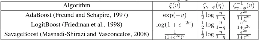
Table 1:Binary losses and correspondingγandφfunctions.
Name ξ(v) γ(v) φ(v)
Exponential exp(−v) v exp(−v)
Logistic log(1 +e−2v) log(1 +v) exp(−2v)
Savage (1+1e2v)2
v
1+v
2
exp(−2v)
4.1.γ−φlosses
Given a set of codewordsY, the optimal multiclass predictorf∗(x)minimizes the classification risk
RLM(f) = EX,C{LM[yc, f(x)]}, (20)
wherecis the class of example x, yc its codeword andLM[yc, f(x)]the loss of predictionf(x).
For classifier design, this is approximated by the empirical estimate
RLM(f) = 1
n
n
X
i=1
LM[yci, f(xi)], (21)
derived from a training sampleD= (xi, ci)ni=1. When the minimization of (21) encourages
predic-tors for which the margin of (14) is large,LM[., .]is denoted amargin loss. This property guarantees
that the optimal predictor has good generalization beyond the training set.
For binary classification, margin losses are monotonically decreasing functions of the margin ycf. The natural multiclass extension would be to consider decreasing functions of the margin, now
defined in (9), i.e.
LM[yc, f(x)] =χ
min l6=c(u
c−ul)
, (22)
with uk as in (11), for some monotonically decreasing function χ. This, however, is a non-differentiable function of the predictorf. We avoid this difficulty by considering the set ofγ−φ losses.
Definition 4 LetY = {y1, . . . , yM} ∈Rdbe a set of codewords,f(x) : X →
Rda predictor. A γ−φloss is defined as
LγM−φ[yc, f(x)] =γ
M
X
l=1,l6=c
φuc−ul
, (23)
whereφ:R→R+andγ :R+→R+are strictly positive andujis defined in (11).
We leave a theoretical discussion of the properties ofγ −φlosses to Section 7. For now, we simply point out that this set includes a large family of losses. In fact, for binary classification with the classic labelsy1=−y2 =−1,u1 =−u2 =−1
2f(x)andL
γ−φ
M [yc, f(x)]reduces to
Lγ2−φ[yc, f(x)] = γ
2 X
k=1|k6=c
φhuc−uki
=γ
φ
(yc−(−yc))f
2
Algorithm 1 CD-MCBoost and GD-MCBoost
Input:Number of classesM, dimensiond, codeword setY ={y1, . . . , yM} ∈Rd, boosting iterationsN and datasetD={(xi, ci)}in=1of examplesxiand class labelsci ∈ {1, . . . , M}.
Initialization: sett= 0, andft= 0∈Rd
CD-MCBoost GD-MCBoost
whilet < Ndo
Computewiwith (29)
forj= 1toddo
Findgˆj(x),αˆj using (39) and (40)
end for
Setj∗ = arg minjR[ft(x) + ˆαjˆg(x)1j]
Updateft+1(x) =ft(x) + ˆαj∗gˆj∗(x)1j
t=t+ 1
end while
whilet < Ndo
Computewi with (29)
Findg∗(x),α∗using (32) and (33) Updateft+1(x) =ft(x) +α∗g∗(x)
t=t+ 1
end while
Output: decision rule:F(x) = arg maxyk
fN(x), yk
whereξ=γ◦φis a composite function. Table 1 shows that the exponential loss of AdaBoost (Fre-und and Schapire, 1997), the logistic loss of LogitBoost (Friedman et al., 1998), and the Savage loss of (Masnadi-Shirazi and Vasconcelos, 2008) can all be interpreted asγ−φlosses with differ-ent choices ofγ andφ. It should be noted that these decompositions are not unique. In all cases,ξ could be equally decomposed intoγ(v) =vandφ=ξ. The key property is thatξis a monotoni-cally decreasing function. In Section 7 we show thatγ−φlosses are margin enforcing wheneverγ is strictly increasing andφis strictly decreasing. This implies thatξ =γ◦φis decreasing.
4.2. Gradient descent
The first boosting algorithm is a gradient descent procedure to seek the optimal predictorf∗(x) = [f1∗(x), . . . , fd∗(x)]of the optimization problem
(
minf(x) RLγ−φ M
[f(x)]
s.t f(x)∈span(H), (25)
whereH={h1(x), . . . , hr(x)}is a set of multivariate weak learners,
hi(x) :X →Rd. (26)
Letft(x) = [f1t(x), . . . , fdt(x)]be the predictor available aftertboosting iterations. At iteration t+ 1,a step is given along the directiong(x)∈ Hof largest decrease of the riskRLγ−φ
M
[f(x)]. This is determined by the directional derivative ofRLγ−φ
M
[f(x)]along the functionalg : X → Rd, at
pointf(x) =ft(x)(Frigyik et al., 2008),
δRLγ−φ M
[ft;g] =
∂RLγ−φ M
[ft+g]
∂
=0
SABERIAN ANDVASCONCELOS
As shown in Appendix B.1,
−δRLγ−φ M [f
t;g] = 1 2n
n
X
i=1
wi
*
g(xi), yci−
X
k6=ci
ykτk(xi, ci)
+
, (28)
where
wi = −γ0
X
k6=ci
φ
1 2
D
ft(xi), yci −yk
E
X
k6=ci
φ0
1 2
D
ft(xi), yci −yk
E
, (29)
and
τk(x, c) =
φ01 2
ft(x), yc−yk P
k6=cφ0
1
2hft(x), yc−yki
. (30)
The direction of steepest descent is the weak learner
g∗(x) = arg min g∈H
δR[ft(x);g(x)] (31)
= arg max g∈H
n
X
i=1
wi
*
g(xi), yci−
X
k6=ci
ykτk(xi, ci)
+
, (32)
and the optimal step size along this direction
α∗ = arg min α∈RRLγM−φ
[ft(x) +αg∗(x)]. (33)
Note thatα∗may not have a closed form and a line search might be required. The predictor is finally updated according to
ft+1(x) =ft(x) +α∗g∗(x). (34)
This procedure is summarized in Algorithm 1-right, and denoted Gradient Descent Multiclass Boosting (GD-MCBoost).
4.3. Coordinate descent
Alternatively, (21) can be minimized by learning a linear combination of scalar functions. In this case, the optimization problem is
(
minf1(x),...,fd(x) RLγ−φ
M ([f1(x), . . . , , fd(x)])
s.t fj(x)∈span(H) ∀j= 1, . . . , d,
(35)
whereH = {h1(x), . . . , hr(x)} is a set ofscalar weak learnershi(x) : X → R. Let ft(x) be the predictor available aftert boosting iterations. At iterationt+ 1 a single componentfj(x)of
f(x) is updated with a step in the direction of the scalar functionalgthat most decreases the risk RLγ−φ
M [f t
along the direction of the functionalg : X → R, at point f(x) = ft(x), with respect to thejth componentfj(x)off(x)
δRLγ−φ M [f
t;j, g] = ∂RLγM−φ[f
t+g1 j]
∂
=0
, (36)
where 1j ∈ Rd is a vector whosejth element is one and the remaining zero, i.e. ft+g1j = [f1t, . . . , fjt+g, . . . , fdt]. As shown in Appendix B.2,
−δRLγ−φ M
[ft;j, g] = −1 2
n
X
i=1
wig(xi)
*
1j, yci−
X
k6=ci
ykτk(xi, ci)
+
, (37)
wherewiis as in (29) andτk(x, c)as in (30). The direction of largest descent is then
g∗(x) = arg min
g∈HδRLγM−φ
[ft;j, g] (38)
= arg max g∈H
n
X
i=1
wig(xi)
*
1j, yci−
X
k6=ci
ykτk(xi, ci)
+
, (39)
and the optimal step size along this direction
α∗ = arg min α∈R
R[ft(x) +αg∗(x)1j]. (40)
Again, this step size may not have a closed form and a line search might be required. The predictor is finally updated with
ft+1 =ft(x) +α∗g∗(x)1j = [f1t, . . . , fjt+α∗g∗, . . . , fdt]. (41)
This procedure is summarized in Algorithm 1-left and denoted Coordinate Descent Multiclass Boosting (CD-MCBoost). In each iteration of CD-MCBoost, the best weak learner update is found for each of thedcoordinates and the coordinate whose update results in the largest reduction of the risk is then chosen. As can be seen from Algorithms 1, MC-Boost algorithms share the simplicity of implementation (a few lines of code) of binary boosting. The main differences between the two are 1) the use of multi-dimensional predictor and codewords, and 2) the weak learner selection rule. We leave an analysis of the role of codewords to Section 5 and consider the weak learner selection rule next.
4.4. Weak learner selection and boosting weights
The update equations of the two MCBoost algorithms are a natural generalization of the update equations of binary boosting. From (32) and (39), the update equation can, in both cases, be written as
g∗(x) = arg max p
1
n
n
X
i=1
wiMˆft(yci, g(xi)) (42)
where
ˆ
Mft(yc, g(x)) = 1 2
*
g(x), yc−X k6=c
τkt(x, c)yk
+
SABERIAN ANDVASCONCELOS
The only difference is that, while for GD-MCBoost g(x)is a generic vector g(x) ∈ Rd, for
CD-MCBoost it is a vector of the formg(x)1j withg(x)∈R. The two algorithms are thus conceptually equivalent. We next show that they are conceptually equivalent to binary boosting algorithms in the sense that they seek, at each iteration, the weak learner of largest margin on a reweighted training sample. The only difference is that MCBoost implements two weighting mechanisms. The first one, implemented through the weightswi, emphasizes difficult examples. The second one, implemented
throughMˆft, emphasizes difficult classes.
When theγ −φloss is margin enforcing, the first weighting mechanism of MCBoost assigns to each example a weight inversely proportional to how well the currently predictor classifies the example. This can be seen by rewriting (29) as
wi = −γ0
X
k6=ci
φ(vk)
X
k6=ci
φ0(vk)
vk=1
2hft(xi),yci−yki
(44)
and using Theorem 5 (see Section 7), which states that a γ −φ loss is margin enforcing when ξ(v) =γ◦φ(v)is a decreasing function. Sinceξ(v)≥0, by definition ofγ−φloss, the derivative ofξ(v)must approach zero for large positive values ofv, i.e. γ0(φ(v))φ0(v)→0for large positive v. Hence,wi is a decreasing function of the margin components< ft(xi), yci −yk >and close
to zero when the smallest component is positive and large. Since, from (9), this implies a large margin, examples of larger margin under the current predictorft(x)will receive smaller weights
than examples of smaller margin. As is common in boosting, this focuses the learning resources in the examples that are poorly classified byft(x). Hence, the first weighting mechanism is the multiclass generalization of the weighting mechanism of binary boosting.
The second weighting mechanism appears onMˆft(yc, g(x)). By rewriting this quantity as
ˆ
Mft(yc, g(x)) = 1 2
X
k6=c
τkt(x, c)hDg(x), yc−ykEi (45)
and comparing to (9), it can be seen thatMˆft(yc, g(x))is an estimate of the marginM(yc, g(x)).
Rather than taking the minimum of the margin componentsg(x), yc−ykover the classesk6=c, this estimate is a weighted average of these components, assigning weightτkt(x, c)to classk. Hence, τkt(x, c)is a weighting mechanism that favors some classes over others. To interpret this mechanism it is useful to consider the case whereφ(v) =e−v and (30) reduces to
τkt(x, c) = e [−1
2hf
t(x),yc−yki]
P
k6=ce
−[1
2hft(x),yc−yki]
= e
[1 2hf
t(x),yki]
P
k6=ce[ 1
2hft(x),yki]
, (46)
the soft-min of (45) approaches the min of (9) asα→ ∞. More generally, up to the approximation of the min by the soft-min operator,
ˆ
Mft(yc, g(x)) = 1 2
X
k6=c
τkt(x, c)hDg(x), yc−ykEi (47)
≈ 1
2hg(x), y
c−yi (48)
where
y = arg min
yj6=ychft(x), y
c−yji= arg max
yj6=ychft(x), y
ji. (49)
This is the multiclass margin of weak learnerg(x)under the alternative margin definitionMˆft(yc, g(x)). Comparing to the original definition of (9), which can be written as
M(yc, g(x)) = 1 2
g(x), yc−y where y= arg min
yj6=ychg(x), y c−y
ji, (50)
ˆ
Mft(yc, g(x))restricts the margin ofg(x) to the worst case codewordy for the current predictor
ft(x). The strength of this restriction is determined by the soft-min operator. If< ft(x), yc−y > is much smaller than < ft(x), yc−yj >, yj 6= y, τkt(x, c) closely approximates the minimum
operator. Otherwise, the remaining codewords also contribute to (45). In summary,τkt(x, c)is a set of class weights that emphasizes classes of small margin forft(x). In addition,Mˆft(yc, g(x))is
an estimate of the margin ofg(x)under the restriction to the most difficult classes for the current predictorft(x). When combined with (29) this leads to a weighting mechanism that emphasizes
difficult examples (through the weightsw) and difficult classes (through the marginMˆft).
4.5. GD vs. CD-MCBoost
Since (29) and (30) only depend on the current predictorft(x)and not on the weak learnerg(x), the computation of weights is identical for GD-MCBoost and CD-MCBoost. The only difference thus resides on the margin estimate of (45). While GD-MCBoost simply chooses the vector weak learnerg(x)with (42)-(45), CD-MCBoost uses
g∗(x) = arg max g∈Hmaxj
1
n
n
X
i=1
wiMˆft(yci, g(xi), j). (51)
In this case, the approximation of (48) is
ˆ
Mft(yc, g(x), j) ≈
g(x) 2 [h1j, y
ci − h1
j, yi] (52)
= g(x)y c j −yj
2 , (53)
andMft(yc, g(x), j)isa measure of the margin ofg(x)under thejthcoordinate of the codewords
that determine the margin of the current predictorft(x).Note that, for binary codewords,
Mft(yci, g(xi), j) ≈
0, ycij =yj yjcig(xi) ycij 6=yj.
(54)
SABERIAN ANDVASCONCELOS
5. Optimal codewords
So far, we have assumed the existence of a good codeword setY ={y1, . . . , yM}. In this section we study the impact of the codeword set on the performance of MCBoost algorithms.
5.1. The role of codewords
In both MCBoost algorithms, the predictor is initialized withf(x) = 0 ∀x, i.e. all examples are mapped to the origin. By minimizing (21), MCBoost then learns a predictor f(x) of maximum margin. From (10), the margin of examplexi is maximal when the projection off(xi)is maximal
along correct class codeword, yci,and minimal along the remaining codewords. If the margin of xi is positive, it can be increased by increasing the magnitude of the projection off(xi)alongyci.
Hence, both MCBoost algorithms seek a predictor f(x) that, for all i, f(xi) 1) is as aligned as
possible with yci and 2) has the largest possible magnitude along this direction. Hence, starting from the origin, both MCBoost algorithmspush all example predictions outward, in the direction of the corresponding class codewords. The effectiveness of this mechanism depends on the structure of the codeword set. For example, if two classes were to share a codeword, it would be impossible to distinguish them with (16) or (17). This implies that some codeword sets result in larger margins for the decision rule of (17) than others.
Intuitively, the margin capacity will increase if the codewords are better separated. This suggests that better performance should be possible for larger values of the codeword dimensiond. However, since increasingdincreases the complexity of the decision rule, there is a trade-off between margin capacity and implementation complexity. For a fixedd, it remains to determine how to best separate the codewords, so as to maximize the margin capacity, and whether a solution to this problem, i.e. an optimal codeword set, exists.
5.2. Optimal codeword sets
To find the optimal set of codewords, we start by noting that there are several factors that impact the margin, (14), of the learned predictor by MCBoost. The first is the complexity and separability of the underlying problem, i.e., if the problem is not separable, there will never be a classifier with
100% accuracy and the margin of (14) will always be negative. The second is the set of weak learners, i.e. if the set of weak learners is limited then the space of their linear combinations won’t be rich enough to have a good classifier. Finally as mentioned above the set of codewords can also impact the margin.
To focus on the impact of the codewords, we assume that 1) the problem is separable and, 2) our weak learners are rich enough and there exists a linear combination of them,f∗, that can separate training examples with100%accuracy. Under these assumptions, according to (14), the margin of f∗ is the positive and we can arbitrarily increase it by increasing norm of f∗. Therefore we can achieve arbitrarily large margin for any codewords set. To resolve this problem we assume that norm off∗is bounded, e.g.,kf∗k= 12.
Definition 5 A predictorf(x)is normalized if||f(x)||= 1,∀x. F is the set of normalized predic-tors.
Finally note that (9) is invariant to the addition of a constant to all codewords. Also if the margin is positive you can arbitrarily increase it by increasing the codewords norms. To remove these issues, we complement the unit norm constraint of (8) with the constraint that the codewords be centered, i.e., add up to zero.
Definition 6 A set of vectorsY ={y1, . . . , yM} ∈Rd, is denoted a centered(M, d)codeword set
if
PM
k=1yk= 0, kykk= 1 ∀k= 1, . . . , M. (55)
The set of all centered(M, d)codeword sets is denotedS(M, d).
In the rest of this section, we assume that codeword sets are always centered, simply referring to a centered(M, d)codeword set as “an(M, d)codeword set,”.
Definition 7 Consider anM-ary classification problem with a codeword setY ∈ S(M, d). The margin capacity ofYis
C[Y] = min
k=1,...,MM(y
k, ξk), (56)
where
ξk= arg max
||v||=1
M(yk, v). (57)
is the predictor direction of largest margin for classk.
The margin capacityC[Y]can then be interpreted as the maximum margin achievable by any predictor inF using codewordsY on any datasetD. Note, from (14), that it is the margin, with respect toY andD, of a predictor which maps all examples from classk into the directionξkof
largest margin. A large capacity implies that the codeword set is such that a large margin can be achieved for all classes. A small capacity implies that there is at least one class for which the largest achievable margin is small. We define the optimal codeword set as that of largest capacity.
Definition 8 Y∗∈ S(M, d)is a codeword set of maximum capacity if
Y∗ = arg max
Y∈S(M,d)
C[Y]. (58)
To formalize this discussion, we start by deriving an upper bound on the margin achievable along any direction of largest margin.
Theorem 1 LetY ∈ S(M, d)be a codeword set with directions of largest marginξk, k∈ {1, . . . , M}
as defined in (57). Then,∀k
M(yk, ξk)≤ M
2(M−1), (59)
Proof See Appendix C.1.
An immediate consequence of (56) and (59) is that, for any codeword setY ∈ S(M, d),
C[Y]≤ M
2(M −1). (60)
SABERIAN ANDVASCONCELOS
Theorem 2 A codeword setY ∈ S(M, d) meets the capacity bound of (60) with equality if and only if its directions of largest margin areξk=yk,∀kand
D
yk, ylE=− 1
M −1 ∀k, l, k 6=l. (61)
Proof See Appendix C.2.
The theorem shows that a codeword set meets the capacity bound if and only if it has the directions of largest margin as codewords. We next derive the conditions under which such a set of codewords exists.
Theorem 3 S(M, d)contains a set of codewords Yc(M, d) that meets the capacity bound if and
only ifd≥M−1. In this case, the codewords inYc(M, d)are the vertexes of a regular simplex in
Rd.
Proof See Appendix C.3.
The proof of the theorem is constructive, providing a procedure to determine the codeword set
Yc(M, d). The main results of this section are summarized in the following corollary, which is a
straightforward consequence of Theorems 1 and 3.
Corollary 3 Let Y∗ be a codeword set of maximum capacity in S(M, d). If d ≥ M −1, the
codewords(y∗)kofY∗ are the vertexes of a regular simplex in
Rd. In this case, the directions of largest margin areξk= (y∗)k,
D
(y∗)k,(y∗)lE=− 1
M−1, ∀k, l6=k (62)
and
C[Y∗] = M
2(M−1). (63)
In summary, the capacity bound of (60) is met whenever d ≥ M −1. Since this bound only depends on the number of classesM, not in the dimensiond, and the decision rule of (17) has linear complexity ind, there is usually no benefit in adopting codewords of dimension larger thanM−1. Hence, when the classification problem has no further constraints, it is natural to rely on codeword sets of dimension
d=M−1. (64)
Figure 1 presents the optimal codeword sets for variousM. Note that in the binary case,M = 2, the optimal codewords are the classical{+1,−1}labels3.
3. A set of Matlab scripts that determine the optimal codeword set for anyMis available at
1 1.5 1 1.5 -0.5 0 0.5 -0.5 0 0.5
-1.5 -1 -0.5 0 0.5 1 1.5 -1.5
-1
-1.5 -1 -0.5 0 0.5 1 1.5 -1.5 -1 1 1.5 1 1.5 -0.5 0 0.5 -0.5 0 0.5
-1.5 -1 -0.5 0 0.5 1 1.5 -1.5
-1
-1.5 -1 -0.5 0 0.5 1 1.5 -1.5 -1 1 1.5 1 1.5 -0.5 0 0.5 -0.5 0 0.5
-1.5 -1 -0.5 0 0.5 1 1.5 -1.5
-1
-1.5 -1 -0.5 0 0.5 1 1.5 -1.5 -1 1 1.5 1 1.5 -0.5 0 0.5 -0.5 0 0.5
-1.5 -1 -0.5 0 0.5 1 1.5 -1.5
-1
-1.5 -1 -0.5 0 0.5 1 1.5 -1.5 -1 1 0 1 -1 0 1 -1 0 1 -1 1 -1 0 1 -1 0 1 -1 0 1
(M = 2, d= 1) (M = 3, d= 2) (M = 4, d= 3)
Figure 1:Codewords of maximal capacity for different values ofM.
5.3. Low-dimensional predictors
Whend < M −1,there is no guarantee that a codeword set of maximum capacity will achieve the capacity bound. Nevertheless, the choice ofd < M −1can be appealing for applications where it is critical to use low-dimensional predictors. In this case, from (9)-(11), (56), (57), and (58), the search for the codeword set of maximum capacity requires the solution of
Y∗= arg max
Y∈S(M,d)k=1min,...,M||maxv||=1minl6=k
hD
yk, v
E
−Dyl, v
Ei
. (65)
This is a non-trivial optimization for which, to the best of our knowledge, there are no efficient algorithms. Hence, it is of interest to consider alternative optimality criteria. One possibility is the max-min codeword distance criterion.
Definition 9 LetYbe a codeword set inS(M, d). The minimum distance ofY is
dmin[Y] = min k,l6=kky
k−ylk2. (66)
Y∗is a max-min distance codeword set inS(M, d)if
Y∗= arg max
Y∈S(M,d)dmin[Y]. (67)
Max-min distance codeword sets have various appealing properties. First, the maximization of dmin[Y]is intuitive. From (17), the decision rule of the maximum margin classifier is based on the
projectionsf, yk
of the predictorf along the codewords. If the codewords are similar, the same will hold for the projections, resulting in lower margins. Second, the problem of (67) is equivalent to determining the maximum diameter ofM equal circles placed on the surface of the unit sphere without overlap. This is known as theTammesproblem (Tammes, 1930). While it does not have closed-form solution, or even a unique solution (any rotation of a valid solution is a valid solution), its numerical solution is much simpler than that of (65). Finally, as shown in the following result, there is a close relationship between the capacity and the minimum distance of any codeword set in
S(M, d).
Lemma 2 LetYbe a codeword set inS(M, d). Then
1
4dmin[Y]≤ C[Y]< 1
SABERIAN ANDVASCONCELOS 1 1.5 1 1.5 -0.5 0 0.5 -0.5 0 0.5
-1.5 -1 -0.5 0 0.5 1 1.5 -1.5
-1
-1.5 -1 -0.5 0 0.5 1 1.5 -1.5 -1 1 1.5 1 1.5 -0.5 0 0.5 -0.5 0 0.5
-1.5 -1 -0.5 0 0.5 1 1.5 -1.5
-1
-1.5 -1 -0.5 0 0.5 1 1.5 -1.5 -1 1 1.5 1 1.5 -0.5 0 0.5 -0.5 0 0.5
-1.5 -1 -0.5 0 0.5 1 1.5 -1.5
-1
-1.5 -1 -0.5 0 0.5 1 1.5 -1.5 -1 1 1.5 1 1.5 -0.5 0 0.5 -0.5 0 0.5
-1.5 -1 -0.5 0 0.5 1 1.5 -1.5
-1
-1.5 -1 -0.5 0 0.5 1 1.5 -1.5 -1 1 0 1 -1 0 1 -1 0 1 -1 0 1 -1 0 1 -1 0 1 -1
(M = 4, d= 2) (M = 5, d= 2) (M = 5, d= 3)
Figure 2:max-min codeword sets for different values ofdandM.
and
dmin[Y]≤ 2M
M−1. (69)
Proof See Appendix D.1.
The following theorem uses this result to show that the optimal codeword sets under the optimality criteria of Definitions 8 and 9 are identical whend > M −1.
Theorem 4 LetY∗ be a codeword set inS(M, d). Ifd ≥ M −1 then Y∗ is a codeword set of
maximum capacity, i.e.
C[Y∗] = M
2(M−1), (70)
if and only ifY∗is a codeword set of max-min distance, i.e.
dmin[Y∗] = 2M
M −1. (71)
Proof See Appendix D.2.
In summary, in the regime of d ≥ M −1, the vertexes of a regular simplex in Rd are both a maximum capacity and a max-min distance codeword sets of S(M, d). These codeword sets achieve both the capacity and max-min distance bounds ofS(M, d). The main difference between the two optimality criteria is the difficulty of finding an optimal solution ford < M−1. While the optimization problem of (65) is difficult, there are many algorithms for the solution of (67). Our implementation uses a solver based on the barrier method (Nocedal and Wright, 1999). Figure 2 presents max-min codewords sets for different values ofM andd.
5.4. Complexity vs. capacity
Hence, for MCBoost, predictor complexity is mostly a function of the predictor dimensiond, not the number of classes. In fact, MCBoost can solve anyM-ary classification problem with a predictor of dimension as low asd = 2. Obviously, this carries a penalty, by limiting the margin capacity of the codeword set. While, as discussed in Theorem 3, the margin capacity can be achieved for any dimensiond ≥ M −1, smaller dimensions typically lead to reduced classification accuracy. Hence, the dimensiondcan be seen as a parameter that controls the trade-off between predictor complexity and accuracy. Note that complexity does not need to refer simply to the number of com-putations. Ford < M, the act of learning the predictorf(x)can be seen as a form of discriminant dimensionality reduction. This could be of interest for applications such as hashing (Datar et al., 2004; Torralba et al., 2008; Kulis and Darrell, 2009; Gong et al., 2012; Liu et al., 2012), where it is important to represent information from many classes by short codes. In this case, MCBoost can directly learn a discriminantrepresentationof low complexity.
6. Weak Learners
In this section, we investigate the role of weak learners in MCBoost. We consider the questions of which weak learner families can be boosted, the role of classification versus real-valued learners, and how these connect to interpretations of boosting as voting rules. While we limit the discussion to GD-MCBoost, for brevity, all considerations extend to CD-MCBoost.
6.1. Boostability
The selection of weak learner family for a boosting algorithm is usually guided by a boostability condition. A weak learner family is boostable if it guarantees zero training error after a sufficient number of iterations of the boosting algorithm. For binary classification, this holds if the family contains a weak learner with better than random performance, i.e. error rate smaller than50%, for any weight distribution over training examples. Existing multiclass boosting algorithms are usually designed for specific classes of weak learners, e.g regression or decision stumps, and require this boostability condition. However, while trivial for binary classification, the “less than chance error” condition can be non-trivial to prove for multiclass problems, where chance level error is M−1 ×100%. For example, (Mukherjee and Schapire, 2013) used a fairly sophisticated game theoretic analysis to derive boostability conditions in terms of the error rate of a set of weak learners. Unlike most of these algorithms, MCBoost has a fairly straightforward boostability condition for any convexγ−φloss. It suffices that, at any iterationt, there exists a weak learnerh∈ Hfor which the directional derivative of (28) satisfies
−δRLγ−φ M
[ft;h]> δ, (72)
for some fixedδ > 0. In this case, it is always possible to reduce the classification risk by adding h to the weak learner ensemble and, by convexity, the algorithm will converge to the minimum training error, which is zero for separable data. In summary, a set of weak learnersHis boostable by MCBoost if, under any weight distribution over training examples, it contains a memberh for which (72) holds withδ >0.
Similarly to binary boosting, this condition can be expressed in terms of the performance of a set of random weak learners. Letρ(x)be a weak learner with random output, i.e.
P(ρ(x) =yk) = 1
SABERIAN ANDVASCONCELOS
It follows that, for any givenxi,i =ρ(xi)is a sample from a random vectoruniformly distributed
over the codeword set{y1, . . . , yM}. The derivative of (28)
−δRLγ−φ M
[ft;ρ] = 1 2n
n
X
i=1
wi
*
i, yci−
X
k6=ci
ykτk(xi, ci)
+
(74)
has expected value
E
n
−δRLγ−φ M
[ft;ρ]o = 1 2n
n
X
i=1
wi
*
E{i}, yci −
X
k6=ci
ykτk(xi, ci)
+
, (75)
Since
E{i}= M
X
k=1
yk
M = 0, (76)
where the second equality follows from (55), it follows that
E
n
−δRLγ−φ M [f
t;ρ]o= 0. (77)
Hence, the boostability condition of (72) can be written as
−δRLγ−φ M
[ft;h]> E
n
−δRLγ−φ M
[ft;ρ]o+δ, (78)
withδ >0. A weak learner family is boostable if, for any weight distribution, it contains a weak learnerhthat beats the random learnerρ. Hence, as is the case for binary boosting, MCBoost can boost any set of any weak learnershwhose performance is slightly better than random, i.e. has “less than1/M×100%error,” for any weight distribution. Note that this result is valid for any setHof weak learners. In fact, the weak learners do not even have to be classifiers. CD-Boost can be applied to any set of real-valued functionsh :X → Rand GD-MCBoost to any set of multi-dimensional functionsh:X →Rd.
6.2. Classification weak learners and voting rules
Obviously, MCBoost can be implemented with classification weak learners. In this case, the algo-rithm can be presented as a voting rule, as in the classical presentation of AdaBoost. In appendix E.1 we derive the GD-MCBoost equations for the case where the weak learner spaceHis a space of multiclass classifiers, i.e.h :X → Y whereY ={y1, . . . , yM}is the codeword set of the classifi-cation problem. We show that, when this is the case, the learned predictor has the form
f(x) = X k
yk X
t|gt(x)=yk
αt (79)
ifYis a codeword set of maximum capacity inS(M, d)and
fk(x) =
X
t|gt(x)=1k
if Y is a set of canonical codewords 1j. In either case, denoting I(g(x) = yk)α as a vote of
strengthαfrom weak learnerg(x)for classk,f(x)can be seen as a weighted average of the class codewords, where each class is weighted by the strength of its weak learner votes.
It is also shown that, although these predictors have different codeword projections, namely
f(x), yj
= X
t|gt(x)=yj
αt− 1
M−1
X
k6=j
X
t|gt(x)=yk
αt, (81)
for the maximum capacity codeword set and
f(x), yj
= X
t|gt(x)=1j
αt (82)
for canonical codewords, the margin components are similar up to a rescaling, namely
D
f(x), yc−yk
E
= M
M−1
X
t|gt(x)=yc
αt−
X
t|gt(x)=yk
αt
, (83)
for a maximum capacity set and
D
f(x), yc−yk
E
= X
t|gt(x)=1c
αt−
X
t|gt(x)=1k
αt (84)
for a canonical set. In summary, for maximum capacity codewords, the projection of f(x) along codeword yj is the difference between the strength of the weak learner votes for class j and the
average vote strength for the remaining classes. Hence, the projection is large if and only if the class receives votes of strength well above average. On the other hand, for canonical codewords, the projection reduces to the strength of the weak learner votes for classj. The margin components are always larger under the maximum capacity codeword set, but the difference vanishes for large M. Nevertheless, due to the similar form of the margin components, the decision rule of (17) is the same in the two cases and consists of choosing the class of strongest vote
F(x) = arg max k
X
t|gt(x)=yk
αt. (85)
The margin condition of (18) thus holds if and only if this is the true classyc.
With regards to learning, it is shown in appendix E.1 that the steepest descent direction of (32) is also
g∗(x) = arg min g∈H
X
i|g(xi)6=yci
wi
1 +
X
j6=ci
τj(xi, ci)I(g(xi) =yj)
, (86)
in the two cases. The weak learner selection rule reduces to selecting the classifierg(x)of lowest error rate on a dataset where each pointxiis reweighted proportionally to how poorly it is classified
by the current predictor ft(x) (which is captured bywi) and the agreement between the
(incor-rect) class to which it is assigned byg(x)andft(x)(captured byP
j6=ciτj(xi, ci)I(g(xi) =yj)).
Note that, even though the weak learner selection rule is identical for the two codeword sets, the algorithms are not the same, since the weightswiandτj(xi, ci)are determined by the margin
SABERIAN ANDVASCONCELOS
6.3. Classification vs. real valued learners
Finally, we consider the question of whether anything is lost by using a set of classification weak learners. Consider the implementation of MCBoost in a spaceHof continuous weak learners. Let the direction of steepest descent of the risk at a given iteration beh(x)∈ H. Then, it is possible to define a classification weak learner
g(x) =yk, k= arg max
j < h(x), y
j > . (87)
It follows that
Z
hg(x), h(x)idx =
Z D
yarg maxj<h(x),yj>, h(x)
E
dx (88)
=
Z
arg max j
h(x), yj
dx. (89)
Sincearg maxj
h(x), yj
≥Dyj+2yl, yjE,∀l6=j, and
yj+yl
2 , y j
=
1
2 ifYis a canonical codeword set 1
2 −
1
2(M−1) ifYis a maximum capacity codeword set,
(90)
the inequalityarg maxj
h(x), yj > 0 holds for both classes of codewords, whenever M > 2. Hence,
Z
hg(x), h(x)idx >0 (91)
andg(x)is a descent direction, albeit not the steepest descent direction, inH. It follows that the family of weak learnersg(x)is boostable. In summary, for either canonical or maximum capacity codeword sets, whenever there is a boostable setHof generic weak learners, there is also a boostable family of classification weak learners, given by (87). The only penalty in adopting the latter is that, because MCBoost is no longer a steepest descent procedure inH, its convergence can be slower.
7. Loss functions
So far, we have considered a generic γ −φloss function. In this section, we derive conditions under whichγ−φlosses belong to some families with desirable properties for classification, such as margin or proper losses. We then design specificγ−φlosses functions in these families and use them to implement different MCBoost algorithms.
7.1. Margin losses
An important question is under which conditions γ −φlosses are margin enforcing, i.e. when the minimization of the empirical risk of a γ − φ loss encourages predictors of large margin
Mp(D, f,Y). The following result shows that this holds whenever γ is strictly increasing and
Theorem 5 Consider a training setD, a codeword setY ={y1, . . . , yM}, a predictorf(x). Let RLγ−φ
M (f)
be the empirical risk of (21) for aγ−φloss as in (23), such thatγ is strictly increasing andφis strictly positive and decreasing. Then
RLγ−φ M
(f) > 1
nγ(φ[Mp(D, f,Y)]), (92) whereMp(D, f,Y)is the margin of predictorf - as defined in (14).
Proof See Appendix F.1.
Sinceγ is strictly increasing andφis strictly decreasing,ξ=γ◦φis strictly decreasing. It follows from (92) that the minimization ofRLγ−φ
M
(f) forces large margins and theγ −φloss is margin enforcing. Note that the minimization of a decreasingξis similar to the definition of margin loss for binary classification, where ξ = γ ◦φis always decreasing. The main difference is that the componentsγ andφnow have different roles. Whileφoperates on each margin component,γ is applied to the aggregate of all the components. Hence, it no longer suffices to specifyξ, butγand φhave to be specified explicitly.
7.2. Proper losses
A loss LM[., .] is said to be proper if it is possible to recover the class posterior probabilities
PC|X(c|x), C = 1, . . . , M, for all x from any predictor f∗(x) optimal under that loss. This
property is important for applications that require a confidence score for the classification. It is natural to ask under which conditions areγ−φlosses proper. For simplicity, we adopt the notation
ηk(x) =PC|X(k|x), (93)
for the posterior class probabilities and represent a codeword set Y = {y1, . . . , yM} ∈ Rd by a
code matrixY∈Rd×M, whose columns are the codewords inY, i.e.
Y = [y1, . . . , yM]. (94)
We also resort to the well known result that, to minimize (20), it suffices to determine the predictor f∗(x)of minimum conditional risk
RLγ−φ M (f
|x) = EC|X{Lγ
−φ M [y
c, f(x)]|x}, (95)
for all x. The following theorem characterizes the set of minimizers of the conditional risk of a γ−φloss.
Theorem 6 LetY = {y1, . . . , yM} ∈ Rdbe a codeword set,f(x) : X →
Rda predictor,ηk(x)
the posterior probabilities of (93), andRLγ−φ M
(f|x)the conditional risk of (95) whenLγM−φ[., .]is a γ−φloss with differentiableγ, φ. In this case any minimizer,f∗, of (95) is a solution of
YQφf∗Γ
γ−φ
f∗ η = 0, (96)
whereY ∈Rd×M is the code matrix of (94),η = [η
1, . . . , ηM]T the vector of posterior
probabili-ties,Qφf,Γγf−φ∈RM×M with
Qφf(k, l) =
−φ0(ul−uk) k6=l
P
j6=kφ
SABERIAN ANDVASCONCELOS
Γγf−φ(k, l) =
(
γ0
P
l6=kφ(uk−ul)
k=l
0 k6=l, (98)
uj as defined in (11) and we have omitted the dependency of all terms onxfor notational simplicity.
Proof See Appendix G.1.
Since (96) holds for any minimizerf∗of (95), the posterior probability vectorηcan be uniquely recovered fromf∗only when the null space ofYQφf∗Γγf−∗φcontains a single probability vector. The
following lemma provides sufficient conditions for this to holds. In the following results, we use
|A|to denote the dimensionality of a spaceA, andRank(A), N ull(A), andRange(A)to denote the rank, null space, and column space of matrixA, respectively.
Lemma 3 LetY = {y1, . . . , yM} ∈ Rd be a codeword set,Y the corresponding matrix of (94)
andQφf,Γγf−φas defined in (97), (98) respectively. The following statements hold.
1. Ifγ :R+→R+is strictly monotonic then
N ull(YQφfΓfγ−φ) =N ull(YQφf) and N ull(QφfΓfγ−φ) =N ull(Qφf).
2. IfRank(Y)≤M −2then|N ull(YQφf)| ≥2
3. IfRank(Y)≥M −1thenN ull(YQφf) =N ull(Qφf).
4. Ifφ:R→R+is strictly monotonic then|N ull(Qφf)|= 1.
Proof See Appendix G.2.
The lemma shows that, ifRank(Y)≥M−1andφ, γare strictly monotonic, the set of vectorsηfor which (96) holds is a one-dimensional space. It remains to verify if this space contains a probability vector, i.e. a vector of non-negative entries that sum to one. The following lemma shows that this is indeed the case.
Lemma 4 Letη = [η1, . . . , ηM]T andQφf,Γγf−φbe as defined in (97) and (98), respectively. If
QφfΓγf−φη= 0then
ηk =
PM
l=1ηlπlφ0(ul−uk)
πkPMl=1φ0(uk−ul)
∀k, (99)
where
πj =γ0
X
l6=j
φ(uj−ul)
∀j. (100)
Furthermore, ifγ :R+ →R+andφ:R→R+are strictly monotonic andη 6= 0then allηkhave
Proof See Appendix G.3.
Together, Lemmas 3 and 4 state that, for any code matrixYsuch thatRank(Y)≥M −1and any pair of strictly monotonic functionsφ, γ, the space ofηthat satisfy (96) is one dimensional and composed by vectors that satisfy (99). Since, for any vectorη6=0in this subspace, allηkhave the
same sign,P
kηk6= 0and thusη¯= Pη
kηk is a probability vector. Under these conditions, the class
posterior probabilities of (96) can be recovered from the optimal predictorf∗as follows.
Theorem 7 LetY ={y1, . . . , yM} ∈ Rdbe a codeword set of matrixY,LγM−φ[., .]aγ−φloss, RLγ−φ
M
(f|x) the conditional risk of (95), andηthe vector of the posterior probabilities of (93). If Rank(Y) ≥M −1and(φ, γ)is a pair of strictly monotonic differentiable functions, thenηcan be recovered from any minimizer,f∗, ofRLγ−φ
M (f
|x)with
η =
Ωγf−φ
−1
e1, (101)
wheree1 = [1,0, . . . ,0]T ∈RM and
Ωγf−φ(k, l) =
1 k= 1
−πlφ0(ul−uk) k6=l
πk
P
j6=kφ
0(uk−uj) k=l,
(102)
withuk,πkas defined in (11) and (100), respectively.
Proof See Appendix G.4
Theorems 3 and 4 show that, for anM-ary classification problem, a codeword space of dimen-sionM−1is the smallest to contain a set of codewords that achieve either the margin capacity or maximum distance bounds. In this case, the optimal codeword set consists of theM vertexes of the regular simplex inRM−1and can be obtained with the procedure of (Coxeter, 1973). The associated matrixYhas rankM−1and the codewords are the directions of largest margin for each of theM classes. Theorem 7 shows that the combination of theM−1dimensional simplex codewords with strictly monotonicγ, φfunctions is a sufficient condition for a properγ −φloss. In this case, the posterior probability vectorηcan be recovered from any minimizerf∗of the risk, using (101).
7.3. Relations to binary classification
A third question of interest is how the results above generalize previously known properties of binary losses. For binary classification, whereM = 2andy1 = −y2 = 1, it follows from (102) that
Ωγf−φ =
1 1
−φ0(u1−u2)γ0(φ(u1−u2)) φ0(u2−u1)γ0(φ(u2−u1)),
=
1 1
−ξ0(f) ξ0(−f),
SABERIAN ANDVASCONCELOS
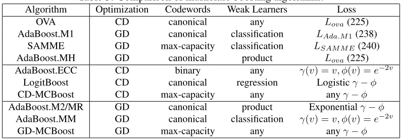
Table 2:Loss, link, and inverse link, of various boosting algorithms.
Algorithm ξ(v) ζγ−φ(η) ζγ−−1φ(v)
AdaBoost (Freund and Schapire, 1997) exp(−v) 12log1−ηη 1+e2ve2v
LogitBoost (Friedman et al., 1998) log(1 +e−2v) 12log1−ηη 1+e2ve2v
SavageBoost (Masnadi-Shirazi and Vasconcelos, 2008) (1+e12v)2 12log η
1−η
e2v
1+e2v
wheref =u1−u2 andξ =γ◦φ. Using (103), the solution of (101) is then
η1 =
ξ0(−f)
ξ0(f) +ξ0(−f) (104)
η2 =
ξ0(f)
ξ0(f) +ξ0(−f), (105)
where we omitted the dependence onx. Definingη=η1, the two equations can be rewritten as
ηξ0(f) = (1−η)ξ0(−f). (106)
This is a popular equation in the binary classification literature, where it is known as a sufficient con-dition forf to minimize the classification risk associated with the binary margin lossξ(.)(Zhang, 2004; Reid and Williamson, 2010). It is usually possible to solve (106) for the optimalf. This is given by
f =ζγ−φ(η), (107)
for some functionζγ−φ, which is denoted the link function of the lossξ. The link function plays an
important role in the recovery of the posterior probabilitiesηkbecause, for a proper lossφ,ζγ−φis
invertible and
η=ζγ−−1φ(f). (108)
Hence, probabilitiesη(x)can be recovered by simply feeding the classifier predictionsf(x)through the inverse of the link. Table 2 lists the loss, link, and inverse link of the margin losses that underlie various popular boosting algorithms.
For M-ary classification, (99) generalizes the inverse link relationship of (108). The main dif-ficulty of the M-ary extension is that the inverse link does not always have closed-form. In fact, while the exact decomposition of the lossξ into the componentsγ andφdoes not affect the link for binary classification, this is not the case forM-ary classification. Consider, for example, the exponential and logistic losses of Table 1. For all these losses,φ(v) =eαv withα∈R−. Consider
next a multiclassγ−φloss whoseφ(.)function is in this family. From (99)
ηk =
PM
l=1ηlπlαeα(u l−uk)
πkPMl=1αeα(u
k−ul)
= e
−αukPM
l=1ηlπleαu l
πkeαu kPM
l=1e−αu
l
![Figure 3: Loss functions Lα[y1, f(x)] for a classification problem with M = 3, d = 2, and the max-capacity code-words of Figure 1 (center), where y1 = (0, 1)](https://thumb-us.123doks.com/thumbv2/123dok_us/9775153.1962758/32.612.103.511.89.289/figure-functions-classication-problem-capacity-words-figure-center.webp)