Numerical Modelling of Trawl Net Considering Fluid-Structure Interaction Based on Hybrid Volume Method

Published by Central Fisheries Research Institute (SUMAE) Trabzon, Turkey in cooperation with Japan International Cooperation Agency (JICA), Japan

R E S E A R C H P A P E R

Numerical Modelling of Trawl Net Considering Fluid-Structure

Interaction Based on Hybrid Volume Method

Yinglong Chen

_{* , Yeming Yao}

1 _{Naval Architecture and Ocean Engineering College, Dalian Maritime University, Dalian 116000, Liaoning, China.} 2 _{Nanjing Engineering Institute of Aircraft Systems, JinCheng, AVIC, Nanjing 211100, Jiangsu, China.}

Article History

Received 27 August 2018 Accepted 27 December 2018 First Online 03 January 2019

Corresponding Author

Tel.: +8641184725229

E-mail: [email protected]

Keywords

Trawl simulation Numerical method Fluid-structure coupling

Abstract

Trawl nets are mostly flexible structures working in the water. In order to investigate the effect of the fluid-structure interaction on the trawl net’s numerical model, we modeled the trawl net and the flow field based on lumped mass method and finite volume method, separately; then we adopted a hybrid volume method (HVM) to model the fluid-structure interaction between the net and surrounding water. Since the gridding of trawl net is independent of its shape within the proposed HVM, large mesh can be used for the calculation of fluid-structure coupling model for higher efficiency. First, existing flume tank experimental data were used to verify the accuracy of the HVM. Then, trawl net states were analyzed based on the HVM by taking the fluid-structure coupling into consideration. The simulation reveals that difference between the trawl net model with and without fluid-structure interaction is about 6%, the main reason for that is the relative velocity of water flow around the codend is only 1/5 of the towing speed because of the flow blocking by the trawl mesh upstream. The above results indicate that fluid-structure interaction is very important for the analysis of trawl net which should not be ignored when numerical modelling.

Introduction

Recent years, with the rising of oil price and global environmental awareness, more and more attention is paid on the fishing efficiency of the trawl net. Usually, field tests can be a reliable way to estimate the behavior the trawl net, but quite expensive both in resources and in time. Besides, it is difficult to change the parameter as freely as you want. In addition to the empirical studies, mathematical modeling is also an effective approach to interpret and predict the motion of trawl net. A number of previous studies can be found to investigate the modeling of the trawl net. Some researchers simplify the trawl net as severally mass

points within the vertical plane to describe the dynamic behavior (Hu et al., 1995, 2001; Lee et al., 2000, 2002; Yonezawa et al., 2009). In order to describe the behavior of the trawl net in space, complex theoretical models for fishing gears are also developed, and the trawl net is composed of huge amount masses that can interpret the shape of the trawl net in detail (Bessonneau et al., 1998; Takagi et al., 2002; Lee et al., 2005; Sun et al., 2011; Khaled et al., 2012; Chen et al., 2014; Yao et al., 2016a; Tang et al., 2017).

hydrodynamic force of the mesh. However, the influence of current on trawl net was usually ignored in the above researches for simplicity. It is necessary to analyze the interaction between trawl net and underwater currents. There are several approaches are adopted to investigate the interaction the net and current including the velocity reduction method and the porous media method. Comparatively speaking, the velocity attenuation method (Løland, 1993; Berstad et al., 2005; Zhan et al., 2006) is too simple to calculate the flow field. Porous media method has been more and more widely used with the improvement of computer ability. Helsley et al. used porous media method to analyze the flow field downstream of the cage and the distribution of nutrients (Helsley et al., 2005). Patursson et al. used the porous medium method to analyze the distribution of the flow field around the mesh at different angles of attack (Patursson et al., 2006), and gave the method to determine the drag coefficient in the porous medium model (Patursson et al., 2010). Zhao et al. used porous media method to study mesh and cage, and pointed out that the thickness of porous media model has little effect on the simulation results (Zhao et al., 2011, 2013a, 2013b, 2015; Bi et al., 2014a, 2014b). However, the porous media method has its own shortcomings, such as the mesh needs to be re-meshed under large deformation. In order to resolve the current net-fluid interaction problems above, Yao et al. (2016b) proposed a novel hybrid volume method to analyze the interaction between the net mesh and the surrounding flow field, which was used to calculate the interaction between the fluid and net cage under large deformation condition.

Within this paper, HVM (Yao et al., 2016b) was adopted to describe the trawl net considering trawl-fluid interaction. The accuracy of HVM was first verified by an experimental case, based on the results calculated by HVM, trawl net states under fluid-solid coupling are analyzed in this paper. The comparison results show that the influence of fluid- trawl coupling on the numerical trawl net model is above 6%, so it is necessary to take the coupling effect of mesh and flow field into account in the modeling of trawl net.

Materials and Methods

The trawl net investigated in this paper is a hexagonal type net produced by Tornet of Iceland (Chen et al., 2014), and it is used for catching Chilean jack mackerel in the fishing ground off Chile. The gear is 496.5 m in length and 1632 m in circumference. The number of net mouth meshes is 68, and the size of net mouth meshes is 24 m. The large meshes are made of Dyneema ropes, and the trawl bag is a polyamide (PA) material. The physical characteristics of the trawl net material are shown in Table 1. The head and foot ropes

are both 387 m in length, and the sinkers mounted on the foot rope are chain with a diameter of 16 mm. A flexible canvas kite is used instead of the floaters for the gear that is mounted on the center of headrope, and it has an effective area of 6.75 m2_{. A rectangular otter} board with an area of 12 m2 _{is adopted on the trawler,} and the weight in water is approximately 22 kN. The weight of the clump mounted on the wings is 12 kN. The diameter of the warps is 32 mm, and the warp weight in water per meter is approximately 28 N. The sweep line made up of wire rope 22mm of diameter and the length is 180m.

Modeling of Trawl Net

In this paper, trawl net is discretized into a series of interconnected spring-mass-damping units based on lumped mass method (Figure 1). External forces, such as hydrodynamics, buoyancy and gravity, are equally distributed to the centralized mass points at both ends of the mesh bar. Similarly, the external forces acting on the board, the lift canvas, and the floats and sinks are concentrated on the points of mass representing them. Therefore, the motion and posture of the net can be simulated by calculating the movement of the concentrated mass point.

Hydrodynamic Force on Knots

Knots of trawl net can be seen as spheres (Takagi et al., 2002, 2004), and the hydrodynamic force acting on knots using Morison equation is written as:

2

1

. 2

kw k Dk k kw

kw

C



  v

H v

v

(1)

where Hk is drag vector, CDkis drag coefficient with

CDk = 1, ρ is fluid density, Ak is the project area of trawl

net knot, vkw is the knot velocity vector relative to water

flow.

Hydrodynamic Force on Ropes

The warps can be assumed to be flexible, slender and elastic ropes, and the mesh bar can be regarded as a single rope with only one point mass in the center. For simplicity, the rope is assumed to be cylindrical element. As for the mesh bar and warp segment, the direction of hydrodynamic force acting on the warp should be considered, and the hydrodynamic force acting on meshes can be described in Figure 2.

The hydrodynamic force on ropes can be divided into the resistance force Fp and tangential viscous force

Ff. Fp is located in the plane composed of umw and ropes

direction vector l, Ff is along with l and has an angle with

the velocity vector umw. The hydrodynamic force Fp and

2

P 90 P

( sin )

. 2



 u

F mw n

N N

C





(2)

2

f f

( cos )

. 2



 u

F mw n

f f

C





(3)

where CN90 is the resistance coefficient in the vertical direction of the rope axis with CN90 = 1.12, Cf is

the viscous friction coefficient with πCf = 1.12 (Zhou et

al., 2014), α is the attack angle of mesh bar, SN and Sf are

the project area and the wet area of the cylinder respectively with SN = dl, Sf = πdl, d and l are the diameter

and length of ropes, np and nf are the unit direction

vectors of Fp and Ff respectively with |np| = 1, |nf| = 1.

Tension Force on Ropes

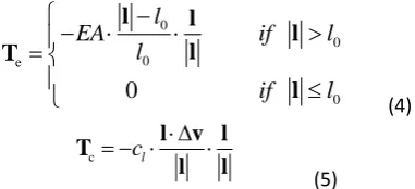
Tension force T acting on the ropes compose of the elastic force Te and damping force Tc. Te is assumed to be

zero force when actual length is less than initial length, Tc changes proportionally with length expand rate. They

can be further written as:

0

0 0

e

0

0

l

EA

if

l

l

if

l















 



_



l

l

l

l

T

l

(4)

c

c



  

l

v l



T

l

l

where E and A are the modulus and cross-section area of ropes, respectively, l is ropes vector (m), l0 is the initial length of ropes (m), cl is the inner damping

coefficient of ropes (N·s/m), Δv is the relative velocity vector between two ends of a rope (m/s).

Considering the process of heaving or shooting the net, it is necessary to deal with the varying length of the warp. Within this paper, the warp is discrete into N elastic warp unit joined at nodes, and number of the nodes N can be altered to change the length of warp. Thus the un-stretched length of warp can be expressed as

Table 1. Parameters of main trawl net components

Material Density/(Kg/m3_{) Young’s modulus /MPa}

Nylon 1150 2830

Dyneema 970 9520

Wire rope 7900 100 000

Figure 1. Lumped mass method of trawl nets.

Figure 2. Definition of hydrodynamic force on ropes. Fp is resistance force vector, Ff is tangential viscous force vector, umw is

 

 

 

 

1

0 0 0

1 0 ₀

+

l t

l

l

t

l

t

r t dt











where l0 is the total payout un-stretched length (m), li0 represent the un-stretched length of the warp unit i (m), with li0 = constant value, lN0 represent the un-stretched length of last warp unit closest to the winch which changes as the winch rotates (m), rw is the rotating speed of trawl winch (m/s), the number of warp units N will increase when lN0 > li0.

Dynamics Equation

According to the analysis of force above, dynamic formula of trawl net can be expressed as：

(m+Δm) a = T+H+W (7)

where a, m, Δm are acceleration vector, real mass and added mass respectively, T, H and W are separately rope tension, hydrodynamic force and weight in water. The added mass of the rope unit can be obtained by:

0 0

0 0

0 0

mt r

r mn r

mb r

C V

m C V

C V         _{  }  

  ₍₈₎

where Cmt, Cmn and Cmb are respectively added

mass coefficients in the direction of t, n and b with Cmt =

0, Cmn = 1 and Cmb = 1, Vr is volume of the mass points.

The added mass of the knot unit can be written as

k m k

m C V

  ₍₉₎

where Vk is the volume knot; Cm is the added mass coefficient with Cm = 0.5.

The weight in fluid of the unit can be given by:

W = (m-ρV) g (10)

where g is the gravity acceleration vector, V is the volume of components including knots, warps and mesh bars.

Modelling of Flow Field

Classic finite volume method was adopted to model the flow field within this paper. Since the fluid in this model is a single component and does not involve heat exchange, the law of mass conservation and momentum conservation are needed to describe the motion of the fluid. The continuity equation of specific volume can be written as：

0

u v w

x y z

 _ _ _

   ₍₁₁₎

where u, v and w are the components of water velocity along the x, y and z coordinate axes. Based on the momentum conservation law, Reynolds-Averaged Navier–Stokes equations are described by:

( )

div( ) +div( _effgrad ) _u

u P

u u S

t x

 _{ }

 

   

 u 

( )

div( ) +div( effgrad ) v

v P

v v S

t y

 _{ }

 _{  } _

 u 

( )

div( ) +div( effgrad ) w

w P

w w S

t z

 _{ }

 _{  } _

 u  ₍₁₂₎

where div represents divergence, grad represents curl of fluid, P can be expressed by the formula p + (2/3)ρk, here p is the pressure and k is the turbulent kinetic energy, μeff is the effective viscosity composed of

dynamic viscosity of water and eddy viscosity, the standard k-ε model is used to calculate the eddy viscosity coefficient, Su, Sv, Sw are the source term, for

incompressible fluid with constant viscosity they are equal to the water resistance force of trawl mesh along u, v, and w direction, and they can be written in equation (13).

Interaction Model of Trawl and Fluid

Hybrid Volume Method

When the trawl moves in water, it will be blocked by the surrounding fluid; at the same time, the mesh will also have a certain effect on the flow. According to Newton's third law, the hydrodynamic force exerted by water flow on the mesh is the same as that exerted by the mesh, and the direction is opposite. In the RANS equation for incompressible fluid with constant viscosity, the source term Si represents the external

force acting on the control volume. Therefore, the drag effect of the theoretical mesh on the fluid can be expressed by adding the hydrodynamic reaction of the mesh structure to the source term of the RANS equation. Based on the above idea, HVM was proposed to solve the coupling effect between the trawl net and fluid (Yao et al., 2016b). Here, the "hybrid volume" indicates that the control volume contains not only fluid information, but also mesh information such as the mesh bar number in the control volume and the proportion of each mesh bar in the control volume.

Discrete Method of Trawl Mesh

hydrodynamic forces of all trawl meshes in hybrid volume, which can be written as:

_

_

[ h, h, h] ( h )

u v w i l i k j

S S S    H  H

(13)

where Su, Sv and Sw are the source terms along x, y

and z directions. Hl_i and Hk_j are the hydrodynamic

forces on the sole i and nodule j respectively, and ξih is

the weight of the sole i in the volume h. The subscript and superscript of ξ indicates the number of the mesh bar or nodule and its volume number respectively. The numbering of knots and mesh bar and the value of mesh bar ξ contained in each hybrid volume can be calculated according to the relative position of bars and knots relative to the space of the computational domain, which is described in detail below.

The computational region and mesh of the flow field in this paper are cuboids which can be seen in Figure 3A. All meshes have the same size. Their length, width and height are Δx, Δy and Δz, respectively. Each grid element uses labels i, j and k to represent its location on the three coordinate axes of x, y and z. The line of A-C-D-B is distributed in the corresponding hybrid volume a-(i, j, k), c- (i-1, j, k) and b- (i-1, j, k+1). Several steps should be conducted to calculate the weight of the mesh bar in the hybrid volume: Firstly, hybrid volume a-(ia, ja, ka) of nodule A and b- (ib, jb, kb) of nodule B are

determined, then according to the direction vector of the trawl mesh, the position (point C) of the mesh bar through the hybrid volume a and the number of the new hybrid volume c- (ic, jc, kc) are calculated. The weight of

the mesh bar AB in the hybrid volume a can be written

as /

a

AB lAC AB

  l

, where lAC is the length of mesh bar AB in hybrid volume a, and lAB is the length vector along

mesh bar. If the incoming hybrid volume c- (ic, jc, kc) is

different from hybrid volume b- (ib, jb, kb), the

intersection point of the mesh bar(point D) and the weight value ξc

AB in the new hybrid volume c are

calculated repeatedly from point C until the hybrid volume of nodule B is reached. After calculating the weights of all the trawl mesh in each hybrid volume, the

source term of RANS equation for each hybrid volume can be calculated by using equation (13), and then the flow field under the action of the mesh can be solved.

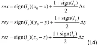
As shown in Figure 3B, the intersection point between the mesh bar and the boundary of the hybrid volume, and the number of the newly entered hybrid volume of the mesh bar can be obtained by the following method. Firstly, according to the direction vector of the mesh bar, the distance between the initial point A and the wall of the hybrid volume in the directions of x, y, z is obtained.

0

0

0

1 sign( ) sign( )( )

2 1 sign( ) sign( )( )

2 1 sign( ) sign( )( )

2

x x

y y

z z

l

rex l x x x

l

rey l y y y

l

rez l z z z



   



   



   

(14)

where sign(i) is a symbolic function, (lx, ly, lz) is the

direction vector of the mesh bar, Δx, Δy, Δz is the length and width of the hybrid volume, (x, y, z) is the spatial coordinate of nodule A, (x0, y0, z0) is the spatial coordinate of the vertex of the hybrid volume and the smallest vertex. The value can be represented by the serial number (i, j, k) of the hybrid volume:

0 0 0

x i x

y j y

z k z

   

   

  

 ₍₁₅₎

By defining the new variables rax = |rex/lx|, ray =

|rey/ly|, raz = |rez/lz|, we can calculate the coordinates

of the intersection point C between the mesh bar and the boundary of the hybrid volume a and the new hybrid volume c- (i-1, j, k). In this paper, o, p and q are used to replace the combination of x, y and z axes, and rao, rap and raq are used to replace the combination of rax, ray, raz. Correspondingly, the parameters [o, p, q, r, s, t] can

represent the following cases by using r, s, t instead of hybrid volume number i, j, k combination.

[ , , , , , ] [ , , , , , ] [ , , , , , ] [ , , , , , ] [ , , , , , ] [ , , , , , ] [ , , , , , ]

x y z i j k x z y i k j y x z j i k o p q r s t

y z x j k i z x y k i j z y z k j i           ₍₁₆₎

According to the relationship among rao, rap and raq, the coordinates of intersection point C (o’, p’, q’) and the ordinal number (r’, s’, t’) of the hybrid volume entered by the mesh bar can be calculated in the following cases.

Case1: when rao < rap < raq or rao < rap = raq, (o’, p’, q’) and (r’, s’, t’) can be written as:





, , ( ) , sign( ) , sign( ) 2      _     _   p q o p q o o l l l

o p q r o p l reo q l reo

l l



 



(17)

Case2: when rao = rap < raq, (o’, p’, q’) and (r’, s’, t’) can be written as:





, , ( ) ( ) , sign( )

2 2       _      _  ，  p q o q o l l l

o p q r o s p q l reo

l









(18)

Case3: when rao = rap = raq, (o’, p’, q’) and (r’, s’, t’) can be written as:





, , ( ) , ( ) , ( )

2 2 2

 

  

  _       _

 

p q

o l l

l

o p q r o s p t q









In the above expressions, lo, lp and lq are the

components of the direction vector l of mesh bar in the direction of o, p and q. By calculating all mesh bar in turn according to the above calculation method, the mesh bar number contained in each hybrid volume and the corresponding hydrodynamic weight of foot in this hybrid volume ξ can be obtained.

In order to consider the influence of the flow field on the mesh, the local water velocity at the nodule

should be used to calculate the hydrodynamic force acting on the mesh. However, when using the HVM to calculate the flow field, the flow velocity calculated by the HVM cannot be directly used to calculate the hydrodynamic force of the mesh, because the flow field grid and the mesh structure are independent of each other. It is necessary to use a certain interpolation algorithm to express the local flow velocity at the nodule with the flow velocity calculated by the HVM, and the details can be found by (Yao et al., 2016b).

Numerical Method

In this paper, the RANS equations of the flow field are discretized by a hybrid scheme, and the pressure-velocity coupling is solved by the Semi-Implicit Method for Pressure Linked Equations (SIMPLE). The coupling between the flow field and the trawl is solved by the iterative computation of the flow field and the mesh model. In other words, the local flow velocity of each node is considered to be constant when the mesh model is calculated, and the position of the mesh in the flow field and the hydrodynamic force on the mesh are considered to be constant when the flow field is calculated.

The coupling between flow field and the trawl mesh can be expressed as follows: (1) Initialization of the computational domain using a uniform flow field; (2) Local flow velocity at each node of the mesh is interpolated according to the existing flow field, and the mesh deformation and hydrodynamics are calculated accordingly; (3) HVM is used to calculate each mixture. (4) Judging the end condition of calculation, if the percentage error of water resistance calculated by two iterations of the mesh is less than 0.1%, the calculation return. If the end condition is not satisfied, the calculation will return to step (2) for a new iteration.

Results and Discussion

In this paper, existing experimental data was used to verify the accuracy of the HVM. The data used in this section are from the measurement experiment of flow field distribution around a rectangular mesh by Bi et al. (2013) using particle image velocimetry (PIV).

Case Description

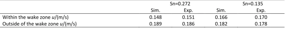
Table 2. Comparison of average water velocity in and outside wake region between simulation and experiments

Sn=0.272 Sn=0.135

Sim. Exp. Sim. Exp.

Within the wake zone u/(m/s) 0.148 0.151 0.166 0.170

Figure 4. The dimension of computational domain and net panel position.

PIV results (m/s) Simulation results (m/s) PIV results (m/s) Simulation results (m/s)

Figure 5. Water velocity distribution comparison between experiments and simulation with Sn=0.272 (A), and comparison results between experiments and simulation with Sn= 0.135 (B).

The width of the flume is 0.45m, and the water depth in the sink is 0.4m for the experiments. The mesh is fixed on the rectangular frame of 0.3m × 0.3m, and the steel frame around the frame is 6mm steel. The frame is fixed in the center of the water tank, the upper edge of the net mouth is homogeneous with the water surface, and the mesh is perpendicular to the water flow direction. The size of the fluid domain and the location of the mesh in the computational domain are shown in Figure 4. The number of grids in the x, y and z directions is 59×21×26.

Bi et al. (2013) carried out experiments on three kinds of density netting at different inlet velocities. In this paper, the test results of 0.272 and 0.135 meshes at 0.17m/s are compared with the simulation results.

Verification Results

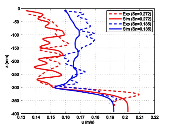
The velocity nephogram of the flow field obtained by experiment and simulation is shown in Figure 5. The section shown in the figure is the plane where the center of the mesh lies. Figure 6 shows the velocity distribution curve in the Z direction of the center plane of the flow field at 150 mm downstream of the mesh. Exp. represents the experimental data and Sim. represents the simulation data.

From Figure 5, it can be seen that there is an obvious wake region downstream of the mesh. The wake region size is basically consistent with the mesh size and keeps a long distance. The simulated wake region is basically consistent with the experimental results. It can also be seen that the velocity fluctuation of the downstream flow of the mesh caused by the discrete distribution of the mesh bar is also reflected in the calculation results.

As can be seen from Figure 6, the velocity in the wake region (the wake region in this section refers to the

region from the horizontal plane to Z = -300mm) decreases with the increase of mesh density, and the velocity outside the wake region increases with the increase of mesh density. When Sn = 0.272, the amplitude of the velocity fluctuation caused by the discrete distribution of the mesh is consistent with the experimental results. For the overall velocity (Table 2), the error between the simulation and experimental results of the average velocity inside and outside the wake region is about 2% of the inlet velocity, which shows that the HVM can calculate the local velocity variation downstream of the mesh very well.

Trawl Net Simulation Analysis

Simulation Description

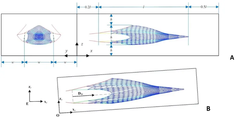
In order to reduce the computational scale of the flow field, the fluid-structure interaction calculation is carried out only after the mesh section of the opponent line. The ratio of the flow field calculation domain to the mesh size is shown in Figure 7A. In the diagram, w is the average opening of the end of the upper and lower grids, h is the vertical opening of the grids, l is the length from the end of the grids to the end of the grids, and the fluid calculation domain is set in proportion to the three base sizes. According to the size of the mesh, the length and width of the fluid domain is about 700m×470m×300m. The number of discrete elements in the length, width and direction of computing domain.

In order to establish the model of mesh and flow field clearly and conveniently, two sets of coordinate systems are adopted in the analysis of fluid-solid coupling problem of trawl mesh: absolute coordinate system { E; xe, ye, ze} and flow field calculation domain

coordinate system { O; xo, yo, zo}. The motion equation

of mesh is established in absolute coordinate system,

Figure 7. Dimensions of trawl net computational domain(A), and the relative relation between coordinate system and absolute coordinate system in computing domain(B).

A

and the coupling model of mesh and fluid is established in the coordinate system of flow field calculation domain. The position relations of the two sets of coordinate systems are shown in Figure 7B. The origin E of the absolute coordinate system is relatively fixed with the trawler, and xe axis is consistent with the velocity

vector of the current relative to the trawler. ze axis is

vertical upward, and ye axis can be given by the

right-hand rule. The origin of O is located at the lower left corner of the front surface of the computational domain. xo axis is consistent with the velocity vector of

water relative to the mesh. zo axis is perpendicular to xo

and obtuse to gravity. yo axis can be given by the

right-hand rule. Because the mesh has high flexibility and its shape changes slowly, it can be considered that the length direction of the mesh is the direction of relative motion between the mesh and the water flow, that is, the direction of xo. In addition, this paper only considers

the direct navigation of trawlers, so the absolute coordinate system {E; xe, ye, ze} and the flow field

calculation domain coordinate system { O; xo, yo, zo } only

rotate around the ye axis at a certain angle except for the

translation relationship.

In this paper, the coordinate values of the end four points (Ps1, Ps2, Ps3, Ps4) and the tail four points (Pw1, Pw2, Pw3, Pw4) of the mesh in the absolute coordinate system are used to calculate the direction of the velocity vector Dfn of water flow relative to the mesh in the absolute coordinate system, and the transformation matrix T from the absolute coordinate system to the computational domain coordinate system：





4 4 4

wi si wi si wi si

P P P P P P

i i i

fn D D D

x x y y z z

x y z   

    

 

 

 

 







D

20)

cos 0 sin 0

0 1 0 0

sin 0 cos 0

1

con con con

x y z

 

 



 

 

 



 

_{  } 

 

T

(21)

where xcon, ycon and zcon are the coordinate values

of the origin of the domain coordinate system in the absolute coordinate system, θ is the angle between the xo axis and the xe axis, cos θ，sin θ can be calculated by

Dfn:

2 2 2 2

cos / ( )

sin / ( )

D D D

D D D

x x z

z x z

 

 

 

(22)

Simulation Results

The simulation results of the flow field around the trawl net are shown in Figure 8. The results of x-y plane and x-z plane in the picture are all shown through the velocity distribution on the axis plane of the mesh. The local velocity of water in the u is normalized by trailing speed u0.

As can be seen from Figure 8, the codend with higher mesh density has a greater effect of blocking water flow, and the relative velocity of water flow and mesh is only one fifth of the towing speed. Therefore, if

Figure 8. Water velocity distribution results around trawl net in 3D view (A), and distribution results around trawl net in in Top view (B).

the towing speed is still used in calculating the hydrodynamic force of this part of mesh, a larger error will occur. For the large mesh, the velocity of the water near the edge of the mesh decreases greatly, which is mainly due to the small angle between the mesh and the water flow and the obstruction of the water flow by multiple mesh. It can also be seen from the diagram that the mesh mainly affects the velocity distribution in the downstream of the mesh, but has little effect on the velocity distribution outside the mesh and upstream of the mesh.

The simulation parameters and the error curves with and without the fluid solid coupling model are shown in Figure 9. The percentage error of the simulation results is defined as follows:

Error = (OutNFSI – OutFSI) / OutFSI × 100% (23)

where OutNFSI is the simulation output of the mesh

model without considering coupling, and OutFSI is the

simulation output of the mesh model with considering coupling.

As seen from the figures, the otterboard spread (Figure 9A), the vertical expansion and the horizontal expansion (Figure 9C, Figure 9D) of the trawl moth increase when considering the coupling effect between the mesh and the flow field. The depth of the trawl increases with the same towing speed and the length (Figure 9B), and the tension decreases (Figure 9E). Considering the fluid-trawl interaction, the deviations of the two simulation results are all about 6% except for the vertical expansion (about 2%). This is mainly due to

considering the fluid-solid coupling, the flow around the small mesh body is blocked by the mesh and moves along with the mesh, so the relative velocity between the flow and the mesh becomes smaller, resulting in the decrease of hydrodynamic force on the mesh.

The decrease of hydrodynamic force enlarges the horizontal and vertical expansion of trawl under the action of otter board and lifting canvas, and the trawl depth becomes deeper under the action of gravity. Therefore, the coupling effect of trawl and flow field should not be ignored. It can also be seen from the graph that the deviation between the simulation results before and after considering the fluid-solid coupling effect is about 4% - 5%, which is smaller than the deviation between the simulation results of the non-release process. The maximum deviation of the two sets of simulation results increased to 8% when the trawl mouth expanded vertically. As seen from the towing curve (Figure 9F), the towing speed decreases with the consideration of the fluid-solid coupling model, which means that the decrease of trawl resistance is not as large as non-release process, which can also be verified by the change curve of traction tension (Figure 9E). However, because the amplitude of drag variation is small relative to the trawler mass, the effect of drag variation on the towing speed is also small (about 1%).

Conclusions

This paper introduces a model of trawl net considering fluid-structure interaction based on HVM. In the HVM, the trawl mesh resistance is obtained directly by the net’s hydrodynamic force which is further discretized in the source term of the N-S equation of the hybrid volume. Flume tank experimental data were used to verify the accuracy of the HVM, and trawl net simulation were then conducted to analyze the performance considering fluid-structure interaction. Some conclusions can be drawn as follows:

(1) The HVM proposed in this paper is independent of the trawl net shape, and it is not necessary to re-mesh the trawl when deformed, and the flow field around the mesh can be calculated by using a sparse mesh. These characteristics make the HVM especially suitable for fluid-structure coupling analysis of meshes with large deformation and irregular shape.

(2) The error between the flow field calculated by the HVM and the experimental results is less than 2%, and the velocity fluctuation in the wake region caused by the discrete distribution of mesh feet can be observed according to simulation results. Therefore, the flow field calculated by the HVM can provide sufficient accuracy and resolution for hydrodynamic analysis of mesh structures.

(3) The coupling effect between trawl net and surrounding water will affect the warp tension, trawl shape and the depth by about 6%. Therefore, the coupling effect between trawl net and water should be

considered in the simulation calculation of trawl net. The simulation results show that the main reason for these deviation is that the flow behind the trawl is obviously blocked by the upstream mesh, and the water velocity is only about 1/5 of the towing speed.

Acknowledgements

This paper is supported by the National Natural Science Foundation of China (51475064) and Fundamental Research Funds for the Central Universities (017183018).

References

Berstad, A. J., Tronstad, H., Sivertsen, S. A., & Leite, E. (2005). Enhancement of Design Criteria for Fish Farm Facilities Including Operations. ASME 2005 International Conference on Offshore Mechanics and Arctic Engineering (pp. 825-832).

Bessonneau, J. S., & Marichal, D. (1998). Study of the dynamics of submerged supple nets (applications to trawls). Ocean

Engineering, 25(7), 563-583.

http://dx.doi.org/10.1016/S0029-8018(97)00035-8. Bi, C.W., Zhao, Y.P., Dong, G.H., Xu, T.J., & Gui, F.K. (2013).

Experimental investigation of the reduction in flow velocity downstream from a fishing net. Aquacultural

Engineering, 57, 71-81.

http://dx.doi.org/10.1016/j.aquaeng.2013.08.002. Bi, C. W., Zhao, Y. P., Dong, G. H., Xu, T. J., & Gui, F. K. (2014a).

Numerical simulation of the interaction between flow and flexible nets. Journal of Fluids & Structures, 45(1), 180-201.

http://dx.doi.org/10.1016/j.jfluidstructs.2013.11.015. Bi, C. W., Zhao, Y. P., Dong, G. H., Zheng, Y. N., & Gui, F. K.

(2014b). A numerical analysis on the hydrodynamic characteristics of net cages using coupled fluid–structure interaction model. Aquacultural Engineering, 59(2), 1-12. http://dx.doi.org/10.1016/j.aquaeng.2014.01.002. Chen, Y. L., Zhao, Y. G., Zhou, H., & Huang, H. L. (2014).

Simulation study of large mid-water trawl system.

Journal of Zhejiang University, 48(4), 625-632.

http://dx.doi.org/10.3785/j.issn.1008-973X.2014.04.010.

Helsley, C. E., & Kim, J. W. (2005). Mixing downstream of a submerged fish cage: a numerical study. IEEE Journal of

Oceanic Engineering, 30(1), 12-19.

http://dx.doi.org/10.1109/JOE.2004.841389.

Hu, F., Matuda, K., Tokai, T., & Kanehiro, H. (1995). Dynamic Analysis of Midwater Trawl System by a Two-Dimensional Lumped Mass Method. Fisheries Science, 61, 229-233. http://dx.doi.org/10.2331/fishsci.61.229. Hu, F., Matuda, K., & Tokai, T. (2001). Effects of drag coefficient

of netting for dynamic similarity on model testing of trawl nets. Fisheries Science, 67(1), 84-89. http://dx.doi.org/10.1046/j.1444-2906.2001.00203.x. Khaled, R., Priour, D., & Billard, J. Y. (2012). Numerical

optimization of trawl energy efficiency taking into account fish distribution. Ocean Engineering, 54(4), 34-45. http://dx.doi.org/10.1016/j.oceaneng.2012.07.014. Lee, C. W., & Lee, J. H. (2000). Modeling of a midwater trawl

Science, 66(5), 851-857. http://dx.doi.org/10.1046/j.1444-2906.2000.00138.x. Lee, C. W. (2002). Dynamic Analysis and Control Technology in

a Fishing Gear System. Fisheries Science, 68(sup2), 1835-1840. http://dx.doi.org/10.2331/fishsci.68.sup2_1835. Lee, C. W., Lee, J. H., Cha, B. J., Kim, H. Y., & Lee, J. H. (2005).

Physical modeling for underwater flexible systems dynamic simulation. Ocean Engineering, 32(3), 331-347. http://dx.doi.org/10.1016/j.oceaneng.2004.08.007. Løland, G. (1993). Current forces on, and water flow through

and around, floating fish farms. Aquaculture

International, 1(1), 72-89.

http://dx.doi.org/10.1007/BF00692665.

Patursson, O. E., Swift, M. R., Baldwin, K., & Tsukrov, I. (2006). Modeling Flow Through and Around a Net Panel Using Computational Fluid Dynamics.Oceans 2006 (pp.1-5). Patursson, Ø., Swift, M. R., Tsukrov, I., Simonsen, K., Baldwin,

K., Fredriksson, D. W., & Celikkol, B. (2010). Development of a porous media model with application to flow through and around a net panel. Ocean

Engineering, 37(2), 314-324.

http://dx.doi.org/10.1016/j.oceaneng.2009.10.001. Sun, X., Yin, Y., Jin, Y., Zhang, X., & Zhang, X. (2011). The

modeling of single-boat, mid-water trawl systems for fishing simulation. Fisheries Research, 109(1), 7-15. http://dx.doi.org/10.1016/j.fishres.2010.12.027. Takagi, T., Suzuki, K., & Hiraishi, T. (2002). Development of the

numerical simulation method of dynamic fishing net shape. Bulletin of the Japanese Society of Scientific

Fisheries, 68(3), 320-326.

http://dx.doi.org/10.2331/suisan.68.320.

Takagi, T., Shimizu, T., Suzuki, K., Hiraishi, T., & Yamamoto, K. (2004). Validity and layout of “NaLA”: a net configuration and loading analysis system. Fisheries Research, 66(2), 235-243. http://dx.doi.org/10.1016/S0165-7836(03)00204-2.

Tang, M. F., Dong, G. H., Xu, T. J., Zhao, Y. P., & Bi, C. W. (2017). Numerical simulation of the drag force on the trawl net.

Turkish Journal of Fisheries & Aquatic Sciences, 17(6), 1219-1230. http://dx.doi.org/10.4194/1303-2712-v17_6_15.

Yao, Y., Chen, Y., Zhou, H., & Yang, H. (2016a). A method for improving the simulation efficiency of trawl based on

simulation stability criterion. Ocean Engineering, 117, 63-77.

http://dx.doi.org/10.1016/j.oceaneng.2016.03.031. Yao, Y., Chen, Y., Zhou, H., & Yang, H. (2016b). Numerical

modeling of current loads on a net cage considering fluid–structure interaction. Journal of Fluids &

Structures, 62, 350-366.

http://dx.doi.org/10.1016/j.jfluidstructs.2016.01.004. Yonezawa, T., Fujimori, Y., Shimizu, S., Kimura, N., & Miura, T.

(2009). Representation of the dynamic characteristics of a towed sampling gear with a linearized model. Nsugaf,

75(3), 390-401.

http://dx.doi.org/10.2331/suisan.75.390.

Zhan, J. M., Jia, X. P., Li, Y. S., Sun, M. G., Guo, G. X., & Hu, Y. Z. (2006). Analytical and experimental investigation of drag on nets of fish cages. Aquacultural Engineering, 35(1), 91-101.

http://dx.doi.org/10.1016/j.aquaeng.2005.08.013. Zhao, Y., Bi, C., Liu, X., Li, Y., & Dong, G. (2011). Numerical

simulation of the flow field around fishing net under current. Proceedings of the Twenty-first International Offshore and Polar Engineering Conference (pp. 963-968). Hawaii, USA.

Zhao, Y. P., Bi, C. W., Dong, G. H., Gui, F. K., Cui, Y., Guan, C. T., & Xu, T. J. (2013a). Numerical simulation of the flow around fishing plane nets using the porous media model.

Ocean Engineering, 62(3), 25-37.

http://dx.doi.org/10.1016/j.oceaneng.2013.01.009. Zhao, Y. P., Bi, C. W., Dong, G. H., Gui, F. K., Cui, Y., & Xu, T. J.

(2013b). Numerical simulation of the flow field inside and around gravity cages. Aquacultural Engineering,

52(52), 1-13.

http://dx.doi.org/10.1016/j.aquaeng.2012.06.001. Zhao, Y. P., Bi, C. W., Chen, C. P., Li, Y. C., & Dong, G. H. (2015).

Experimental study on flow velocity and mooring loads for multiple net cages in steady current. Aquacultural

Engineering, 67, 24-31.

http://dx.doi.org/10.1016/j.aquaeng.2015.05.005. Zhou, C., Xu, L., Zhang, X., & Ye, X. (2014). Application of

Numerical Simulation for Analysis of Sinking Characteristics of Purse Seine. Journal of Ocean

University of China, 14(1), 135-142.