Vol. 15, No. 2, 2017, 185-192
ISSN: 2279-087X (P), 2279-0888(online) Published on 11 December 2017
www.researchmathsci.org
DOI: http://dx.doi.org/10.22457/apam.v15n2a4
185
Annals of
Paradox in a Linear Multi Objective Transportation
Problem
R. Sophia Porchelvi1 and M. Anitha2 A.D.M. College for Women (Autonomous)
Nagapattinam–611 001, Tamil Nadu, India 1
Email: [email protected]; 2Email: [email protected]
Received 1 November 2017; accepted 9 December 2017
Abstract. In this paper, an algorithm is developed to find the paradoxical solution of multi objective transportation problem with linear constraints. It also attempts to obtain its best paradoxical pair and paradoxical range of flow by using the sufficient condition of the existing paradox. Numerical illustration is also provided to check the feasibility.
Keywords: Northwest corner method, Multi objective transportation problem, Paradoxical pair, Paradoxical range of flow.
AMS Mathematics Subject Classification (2010): 90C08 1. Introduction
The term Paradox arises when a transportation problem admits a total cost which is lower than the optimum. This is attainable by shipping larger quantities of goods over the same routes that were previously chosen as optimal which is unusual phenomenon noted by Szwarc (1971). The classical transportation problem is the name of a mathematical model has a special mathematical structure. The mathematical formulation of a large number of problems conforms to this special structure. Hitchcock (1941) originally developed the basic linear transportation problem. Klingman and Russel (1974 and 1975) introduced a specialized method for solving a transportation problem with several additional linear constraints. Hadley (1987) gave the detailed solution procedure for solving linear transportation problem. Till date, several researchers studied comprehensively to solve transportation problem cost minimizing its cost in various ways.
186
This Paper is organized as follows: In Section 2 Basic Definitions are given. Section 3 explains the mathematical formulation and sufficient condition for the existence of paradox of linear Multi objective transportation problem. In Section 4, an Algorithm is developed to solve linear Multi objective transportation problem. In Section 5, a Numerical Example is given to show the optimal solution of linear Multi objective transportation problem. In that solution, the paradoxical range of the flow and the best paradoxical pair is found. The conclusion of the paper is given in Section 6.
2. Preliminaries
Paradox in a transportation problem: In a transportation problem if we can obtain more flow (F1) with lesser cost (Z1) than the optimum flow (F0) corresponding to the optimum cost (Z0) i.e.F1> F0 and Z1< Z0, then we say that a paradox occurs in a transportation problem.
2. Cost-flow pair: If the value of the objective function is Z0 and the flow is F0 corresponding to the feasible solution X0 of a transportation problem, then the pair corresponding to the feasible solution X0.
3. Paradoxical pair: A cost-flow pair, (Z,F) of an objective function is called paradoxical pair ifZ< Z0and F>F0 where Z0 is the optimum cost and F0 is the optimum flow of the transportation problem.
4. Best paradoxical pair: The paradoxical pair(Z*, F*) is called the best paradoxical pair of a transportation problem if for all paradoxical pair (Z, F), either Z*< Z or Z*=Z but F*>F.
5. Paradoxical range of flow: If F0 be the optimum flow and F* be the flow corresponding to the best paradoxical pair of a transportation problem then [F0, F*] is called paradoxical range of flow.
3. Mathematical formulation
Consider the following linear Multi-Objective Transportation problem (LMOTP) (P1): Minimize Z = ∑(,)∈,∑(,)∈,… … . ∑(,)∈,
Subject to ∑∈ = , i∈
∑∈ = , j∈
Xij ≥ 0∀ (, ) ∈
where ai is the ith source, bj is the jth destination
Xij= the amount transported from the ith source to the jth destination.
Clij = the cost per unit amount transported from ith source to the destination corresponding to k objectives. i.e. l=1, 2,3,...k.
In this paper we assume that ai> 0, i∈ and >0, j∈ and ∑!"#= ,∑"#= , Let X0= {$\ (i,j) ∈ I x J} be a basic feasible solution corresponding to the basis B of the problem P1 and the value of the objective function Z1,2,...k corresponding to the basic feasible solution X0 is given below.
187 Let F0 be the corresponding flow.
Then F0 = ∑ ∈% = ∑∈%.
Let (ULi , VLj), (L=1,2,3....k) be the corresponding dual variable associated with the above k problems (Pl), so that UiL + VLj = CLij for (i, j)∉ B ∀ L= 1,2,3,....k.
Let CLij = (UiL+VLj) - Cij
If CLi j< 0 for (i , j) ∉ B ∀L=1,2,3,...k, then the solution is optimal.
Theorem 1. The sufficient condition for the existence of paradoxical solution of (P1) is that if ∃ at least one cell (r,s) ∉ B in the optimum table of (P1) where arand bs are replaced by ar+ l and bs+ l respectively(l>0) then (UiL + ViL) < 0, L=1,2,3...k.
Proof: Let Z1,2,3...k be the value of the objective function and F1,2,3....k be the optimum flow corresponding to the optimum solution X1,2,3,...k of problem P1. The dual variables UiL and ViL are given by
UiL+ ViL = Cij , (i , j) ∈J
Then, Z1= ∑(,)∈ , Z2 = ∑(,)∈ ,… … … Zk = ∑(,)∈ and F0 = ∑"#= ∑!"#
Now, let ∃ at least one cell (r,s) ∉ B, where ar and bs are replaced by ar+ l and bs+ l respectively (l>0) in such a way that the optimum basis remains same, then the value of the objective function Z is given by
Z = [ Z0 + l (UiL + ViL)] The new flow F is given by
F = ∑"# + l = ∑!"# + l = F0 + l F - F0 = l > 0
Therefore, for the existence of paradox we must have Z –Z1,2,3,...k< 0.Hence the sufficient condition for the existence of paradox is that ∃ at least one cell (r,s) ∉ B in the optimum table such that if ar and bs are replaced by ar + l and bs + l respectively. Then ( l> 0) then l(UiL + ViL) < 0, L=1,2,3...k.
(i.e) (UiL + ViL) < 0, the solution is optimal.
4. Algorithm for solving linear multi objective transportation problem Step 1: Find the cost-flow pair (Zi ,Fi) for the optimum solution X0, (i= 1,2,3,...k)
Step 2: Fix i=1
Step 3: Find all cells where (r, s) ∉ B such that (Ur +Vs) <0 if it exists otherwise go to step 8.
Step 4: Among all cells (r, s) ∉ B satisfying step 3 find min flow for l=1 which enter into the existing basis whose corresponding cost is minimum. Let (Zi,Fi) be the new cost flow pair corresponding to the optimum solution Xj (j= 1,2,...k)
Step 5: Write ( Zj, Fj).
188 Step 7: Repeat the procedure goto step 3.
Step 8: We write the best paradoxical pair (Z* ,F*) = (Zj, Fj) for the optimum solution X* =Xj.
Step 9: Finding the paradoxical solution, end at this stage.
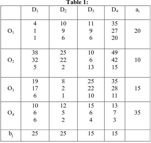
5. Numerical illustration
Consider the following Multi objective linear transportation problem using the numerical values, as tabulated below:
Table 1:
D1 D2 D3 D4 ai
O1 4 1 1 10 9 6 11 9 6 35 27 20 20 O2 38 32 5 25 22 2 10 6 13 49 42 15 10 O3 19 17 6 8 2 1 25 22 10 35 28 11 15 O4 10 6 6 12 5 2 15 6 4 13 7 3 35
bj 25 25 15 15
Solving the above problem using the Northwest corner method, the optimal Multi objective transportation table is presented in Table II.
Table II: D1 b1=25 D2 b2=25 D3 b3=15 D4 b4=15
U1i U2i U3i
O1: a1= 20 4 1 1 (20) 0 0 0
10 9 6
-9 -9 -2
11 9 6
-6 -8 0
35 27 20
-8 -7 -1
-21 -14 -4
O2: a2= 10 38 32 5 (5) 0 0 0
25 22 2 (5) 0 0 0
10 6 13
28 23 4
49 42 15
26 24 3
189 O3: a3= 15 19 17 6
21 12 4
8 2 1 (15) 0 0 0
25 22 10
11 3 3
35 28 11
9 4 2
-4 -3 -1
O4: a4= 35 10 6 6
25 15 5
12 5 2 (5) 0 0 0
15 6 4 (15) 0 0 0
13 7 3 (15) 0 0 0
0 0 0
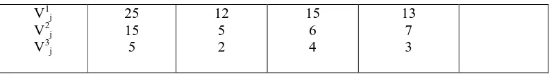
V1j V2j V3j
25 15 5
12 5 2
15 6 4
13 7 3
For this solution is X= {20, 0, 0, 0, 5, 5, 0, 0, 0, 5, 0, 0, 0, 5, 15, 15} for which Z = (995,540,185), Z1=995, Z2=540, Z3=185.
When we check the sufficient condition for the existence of paradoxical solution (Ur+ Vs) where(r, s) ∄ B in Table 1, we observe that for Z1, a paradox occurs in the cell (1,2)(1,3)(1,4) but not in (2,3),(2,4),(3,1),(3,3),(3,4),(4,1).
Next Z2, a paradox occurs in the cell (1,2)(1,3)(1,4) but not in (2,3),(2,4),(3,1), (3,3), (3,4),(4,1).
Next Z3, a paradox occurs in the cell (1,2),(1,4) but not in (1,3), (2,3), (2,4), (3,1), (3,3), (3,4) and (4,1).
Hence Z1, Z2, Z3 the paradox occurs commonly in the cell (1,2) and (1,4).
Applying Step 1: The cost flow pair is (995, 540, 185) (80, 80, 80) corresponding to the optimum solution X0 = {X11= 20, X21 =5, X22 = 5, X32 =5, X42 = 5, X43 = 15, X44 = 15} Step 2: Fix i=1
Step 3: Now check the sign of Ur+ Vs and we obtain for the non-basic cells (1, 2) and (1, 4), the sign that is negative.
Step 4: Hence consider l=1 enters in to the optimum basis for the cell (1, 2)
Table III: D1
b1=25
D2
b2=26
D3
b3=15
D4
b4=15
U1i U2i U3i
O1: a1= 20 4 1 1 (21)
10 9 6 11 9 6 35 27 20
-21 -14 -4
O2: a2= 10 38 32 5 (4)
25 22 2 (6)
10 6 13 49 42 15
13 17 0
O3: a3= 15 19 17 6 8 2 1 (15)
25 22 10
35 28 11
-4 -3 -1
O4: a4= 35 10 6 6 12 5 2 (5)
15 6 4 (15)
13 7 3
190 V1j
V2j V3j
25 15 5
12 5 2
15 6 4
13 7 3
The corresponding paradoxical pair is (986, 531,183) (81, 81,81).
For the cell (1,4)Multi objective transportation table is presented in Table IV
Table IV: D1
b1=25
D2
b2=25
D3
b3=15
D4
b4=16
U1i U2i U3i
O1: a1= 20 4 1 1 (21)
10 9 6 11 9 6 35 27 20
-21 -14 -4
O2: a2= 10 38 32 5 (4)
25 22 2 (6)
10 6 13 49 42 15
13 17 0
O3: a3= 15 19 17 6 8 2 1 (15)
25 22 10 35 28 11
-4 -3 -1
O4: a4= 35 10 6 6 12 5 2 (4)
15 6 4 (15)
13 7 3
(16) 0 0 0
V1j V2j V3j
25 15 5
12 5 2
15 6 4
13 7 3
The corresponding paradoxical pair is (987, 533,184) (81, 81,81) The min cost = {(986, 531, 183), (987, 533, 183)} = (986, 531, 183).
Hence l=1 enters in the optimum basis from the cell (1, 2) and corresponding table is Table IV, the corresponding paradoxical pair is (986, 531, 183) (81, 81, 81). Repeating this process in the next table
Table V: D1
b1=25
D2
b2=27
D3
b3=15
D4
b4=15
U1i U2i U3i
O1: a1= 20 4 1 1 (22)
10 9 6 11 9 6 35 27 20
-21 -14 -4
O2: a2= 10 38 32 5 (3)
25 22 2 (7)
10 6 13 49 42 15
13 17 0
191
(15) -4 -3 -1
O4: a4= 35 10 6 6 12 5 2 (5)
15 6 4 (15)
13 7 3
(16) 0 0 0
V1j V2j V3j
25 15 5
12 5 2
15 6 4
13 7 3
The corresponding paradoxical pair is (977, 522, 181) (82, 82, 82)
Henceforth from the final Table-VI the best paradoxical pair and the paradoxical range of flow showing an increase in the flow within the value of the objective function, and thus decreases from the optimal solution of the Multi Objective linear transportation problem.
Table VI: D1
b1=25
D2
b2=30
D3
b3=15
D4
b4=15
U1i U2i U3i
O1: a1= 20 4 1 1 (25)
10 9 6 11 9 6 35 27 20
-21 -14 -4
O2: a2= 10 38 32 5 (0)
25 22 2 (10)
10 6 13 49 42 15
13 17 0
O3: a3= 15 19 17 6 8 2 1 (15)
25 22 10 35 28 11
-4 -3 -1
O4: a4= 35 10 6 6 12 5 2 (5)
15 6 4 (15)
13 7 3
(15) 00 0
V1j V2j V3j
25 15 5
12 5 2
15 6 4
13 7 3
The corresponding paradoxical pair is (950, 495,175) (85, 85, 85)
Applying step 8: The best paradoxical pair is (Z*, F*) = {(950, 495, 175) (85, 85, 85)}. Corresponding to the optimum solution X0 = {X11= 25, X21 =0, X22 = 10, X32 =15, X42 = 5, X43 = 15, X44 = 15} and the paradoxical range of flow is [F0, F*] = (80, 80, 80) (85, 85, 85).
6. Conclusion
192 REFERENCES
1. D.Acharya, M.Basu and M.Das, More-for-less paradox in a transportation problem under fuzzy environments, J Appl Computant Math., 4 (2015) 202.
2. V.Adlakha and K.Kowalski, A quick sufficient solution to the more-for-less paradox in a transportation problem, Omega, 26(4) (1998) 541-547.
3. G.M.Appa, The transportation problem and its variants, Operations Research.Q. 24 (1973) 79-99.
4. M.Basu, D.Acharya and A.Das, The algorithm of finding all paradoxical pair in a linear transportation problem, Discrete Mathematics, Algorithm and Application, 4 (2012) 1250049 (9 pages).
5. A.Charnes and D.Klingman, The more-for-less paradox in the distribution model,
Cachiersdu Centre Etudes de Recherche Operaionelle, 13 (1971) 11-22.
6. V.G.Deineko, B.Klinz and G.J.Woeginger, Which matrices re immune against the transportation paradox?, Discrete Applied Mathematics, 130 (2003) 495-501.
7. A.Gupta, S.Khanna and M.C.Puri, A paradox in linear fractional transportation problems with mixed constraints, Optimization, 27 (1993) 375-387.
8. F.L.Hitchcock, The distribution of a product from several resources to numerous localities, Journal of Mathematical Physics, 20 (1941) 224 – 230.
9. V.D.Joshi and N.Gupta, On a paradox in linear plus fractional transportation problem, Mathematika, 26(2) (2010)167-178.
10. S.Storoy, The transportation paradox revisited, N-5020 Bergen, Norway, (2007). 11. W.Szwarc, The transportation paradox, Nav. Res. Logist. Q., 18 (1973) 185-202. 12. D.J.Vishwas and G.Nilama, On a paradox in linear plus linear plus linear fractional