Scheduling Single-Load and Multi-Load AGVs in Container Terminals

Scheduling Single-Load and Multi-Load AGVs in

Container Terminals

Hassan Rashidii

Received 29 April 2009; received in revised 4 August 2009; accepted 22 September 2010

i Corresponding Author, H. Rashidi is with the Department of Mathematics, Statistics and Computer Science, Allameh Tabataba’i University, Tehran, Iran (Email: [email protected])

ABSTRACT

In this paper, three solutions for scheduling problem of the Single-Load and Multi-Load Automated Guided Vehicles (AGVs) in Container Terminals are proposed. The problem is formulated as Constraint Satisfaction and Optimization. When capacity of the vehicles is one container, the problem is a minimum cost flow model. This model is solved by the highest performance Algorithm, i.e. Network Simplex Algorithm (NSA). If the capacity of the AGVs increases, the problem is a NP-hard problem. This problem has a huge search space and is tackled by the Simulated Annealing Method (SAM). Three approaches for its initial solution and a neighborhood function to the search method are implemented. The third solution is a hybrid of SAM and NSA. This hybrid is applied to the Heterogeneous AGVs scheduling problem in container terminals. Several the same random problems are generated, solved by SAM with the proposed approaches and the simulation results are compared. The experimental results show that NSA provides a good initial solution for SAM when the capacity of AGVs is heterogeneous.

KEYWORDS

Simulated Annealing Method, Network Simplex Algorithm, Optimization methods, Container Terminals

1. INTRODUCTION

In the past few decades, much research has been devoted to technology of Automated Guided Vehicle (AGV) systems, both in hardware and software (see [18-21]). Nowadays they have been become popular over the world for automatic material-handling and flexible manufacturing systems. These unmanned vehicles are also increasingly becoming common mode of container transport in the seaport. In this paper, we consider a highly automated seaport container terminal, which consists of a berthing area (quay-side), an AGV area, and a storage area (yard-side). Figure 1 illustrates the layout of one of the latest seaport container terminals. The berthing area is equipped with quay cranes for the loading and unloading of vessels. The storage area is divided into blocks each of which is serviced by one or more stacking cranes. The transportation of the containers from the berthing area to the storage area is realized by AGVs, which can carry up to two 20ft containers or alternatively one 40 or 45ft container at a time. In the container terminal considered, AGVs are operated in single-carrier mode, but shall be used as multi-load carriers in the future.

This paper is motivated by a need to dispatch a number

of Automated Guided Vehicles (AGVs) in the container terminals. The AGV dispatching usually consists of three sub-problems, namely assigning AGVs to transportation orders, routing the AGVs, and traffic control. Generally, algorithms for routing and traffic control are already included in the control software provided by the AGV manufacturer. Therefore, only the assignment problem is considered in this paper. The problem requirement in the port is described by a set of jobs, where each job is characterized by the source location of a container, the target location and the time of its picking up or dropping-off on the quay side by the quay crane. Given a number of AGVs and their availability, the task is to assign the AGVs to meet the transportation requirements.

Figure 1: Layout of a seaport container terminal [5]

2. RELATED WORK

Qiu et al. (2002) provided a survey of scheduling and routing algorithms for automated guided vehicles (AGVs) [18]. The authors showed similarities and differences between scheduling and routing AGVs and related problems like the vehicle routing problem, the shortest path problem and scheduling problem. The authors classified algorithms in groups for general path topologies, for path optimization, for specific path topologies and dedicated scheduling algorithms. In the general path topologies, the methods adopted have been classified into three categories: (a) Static methods (b) Time-window-based methods and (c) Dynamic methods. The survey showed that most of the existing solution methods are applicable to systems with a small number of AGVs, offering a low degree of concurrency.

During the recent years, several researches have been devoted on dispatching of vehicles in the port. Huang and Hsu (2002) presented two integer programming models for dispatching vehicles to accomplish a sequence of container jobs from quay-side to yard-side [9]. In the models, the order of vehicles for carrying out the jobs needed to be determined. Two heuristic algorithms were constructed based on the two integer programming models. Using a formulation as the Lagrangian relaxation dual problem, the authors provided a lower bound for the objective function of the second model. Numerical results of the two heuristic algorithms, applied to a real size virtual terminal, were reported. Based on the second model, the author derived a formula to determine the optimum number of vehicles to handle a sequence of container jobs.

Böse et al. (2000) focused on the process of container transport by quay cranes and straddle carriers between the container vessel and the container yard [21]. The objective was reduction of the time in port for the vessels

by maximizing the productivity of the quay cranes. The authors investigated dispatching approaches for straddle carriers to quay cranes in order to minimize vessel’s turnaround time. The author presented an evolutionary algorithm to solve the problems and did a simulation for real data. The results showed that the influence of the number of sequenced containers is not a major concern in the dynamic assignment when the carriers operate in the double-cycle mode.

Wook and Hwan (2000) applied two different dispatching strategies for AGVs in container terminals [2]. In the first strategy (known as dedicated dispatching), every AGV is assigned to a single QC. In the second one, known as pooled dispatching, an AGV performs delivery tasks for more than one QC. The author made integer programming models and tackled them by LINDO software. The research showed that the "pooled dispatching" is preferred over the "dedicated dispatching". Qiu and Hsu (2000-1) addressed scheduling and routing problems for AGVs [18] and developed conflict-free routing algorithms for two different path topologies and two scheduling strategies. The routing efficiency was analyzed in terms of the distance travelled and the time required for AGVs to complete all pickup and drop-off jobs. The research showed that a high degree of concurrency of AGV moves could be achieved, although the routing decision took only a constant amount of time for each vehicle.

compared with the current scheme at a terminal in Singapore, in a simulation experiment. Analysis of the results showed that the algorithm makes improvements in throughput of the terminal.

Cheng et al. (2003) studied dispatching automated guided vehicles in a container terminal [12]. The authors presented a network flow formulation to minimize the waiting time of the AGVs on the berth side. In a similar paper concerning the same project, Chan [13] models a network flow in order to develop an efficient dispatching strategy for AGVs. In the model, the constraints described disparate instances of AGVs to carrying one container or two containers. The author proposed a heuristic algorithm and tested it in case of single load AGV, compared with the current deployment strategy in a port. The results showed some improvements by the model and algorithm in a case study of Singapore port for 20 AGVs and 16 quay cranes.

Grunow et al. (2004) studied dispatching multi-load AGVs in highly automated seaport container terminals [5]. They made a Mixed Integer Linear Program (MILP) model and presented some priority rules to handle container jobs in the container terminals. Then, the performance of the priority rule based approach and the MILP model have been analyzed for different scenarios with respect to total lateness of the AGVs. The main focus of their numerical investigation was on evaluating the priority rule based approach for single and dual-load vehicles as well as comparing its performance against the MILP modeling approach for two layouts(small and large) of a virtual port. In the larger layout, the research considers 6 Dual-Load AGVs and 6 quay cranes.

Murty et al. (2005) presented an integrated approach. The authors proposed a decision support system [6] for operations in a container terminal, focusing on a system that reacts adequately to changes in the workloads over time and to uncertainty in working conditions. One of the functions in the decision support system was to estimate of the number of vehicle required each half-hour and to hire the minimum number of vehicles over a planning horizon of each day. At the end of each planning period, the system used the latest information for the next period. Following the practice of the terminals in Hong Kong, the authors proposed a planning period of 4 hours (i.e. half of an 8-hour shift) since the work loads could be estimated with reasonable accuracy over the period.

Rashidi and Tsang (2005) also studied dynamic scheduling of Single-Load AGVs in container terminals[14]. The problem was formulated as a minimum cost flow model. The authors considered three terms in the objective function: (a) traveling time of the AGVs in the route of terminal; (b) waiting time of the AGVs on the berth-side; and (c) the lateness of serving the container jobs. To solve the problem, the authors extended the standard network Simplex Algorithm (NSA) and obtained

a novel algorithm, NSA+. To complement NSA+, the authors presented an incomplete algorithm, Greedy Heuristic Search (GHS). To evaluate the relative strength and weakness of NSA+ and GHS, the two algorithms were compared for the dynamic automated vehicle scheduling problem.

3. PROBLEM DEFINITION AND FORMULATION

In this section, the AGV scheduling problem in the container terminals is defined and formulated. The most important reason for choosing this problem is that the efficiency of a container terminal is directly related to the use of the AGVs with full efficiency

A. Assumptions

The assumptions used here, is very similar to the assumptions in , i.e. the difference is only in the capacity of the AGVs. That paper assumed that the AGVs are homogenous with unit capacity, but here we assume that they are heterogeneous. In formal, we substitute the Assumption-4 in with the following:

Assumption-4: We are given a fleet of V={1,2,..,|V|} vehicles. The vehicles are heterogeneous and every vehicle transports a few containers. At the start of the process, the vehicles are assumed to be empty.

B. Formulation

The Assumption-4 converts the problem in into an NP-hard problem; however the formulation, here, is completely different. The formulation in is an MCF model, whereas the problem, here, is formulated as Constraint Satisfaction and Optimization (CSOP).

A directed graph or network is considered for this transportation system. Given n for the number of jobs, let node i and node n+i represent the pickup and delivery location of the ith job in the network, respectively. In this network, different nodes obviously may represent the same physical location in the yard or berth. By adding node 0 and node 2n+1, as the depot, to the network, the node set becomes N={0,1,2,..,n,n+1,n+2,..,2n, 2n+1}. The pick up and delivery points are respectively included into two sets P+={1,2,..,n} and P- ={n+1,n+2,..2n}. Obviously P = P+U _P

is the set of nodes other than the depot node. The following parameters are known:

ATj: The appointment time of the jth job.

TSvo : The times at which the vehicle v leaves the depot.

qv: The capacity of vehicle v.

TTij : The travel time from the physical location of node i, Li , to physical location of node j , Lj (for each pair of i, j in N).

I) Decision variable

Xijv : This variable is 1 if vehicle v moves from node i

to node j; otherwise, it is 0.

II) Constraints and Objective function

need a couple auxiliary variables. The first one, Yvi , is the

load of vehicle v when it leaves node i. At the start of the process Yv0=0. This variable is determined by the

equations set (1). The first statement in the equations set (1) represents the load of a vehicle when it leaves the first pickup point after the depot. The second statement in the equations set (1) has a similar meaning but for when each vehicle goes to any pick up or drop-off point after the first pickup. If a vehicle goes to any pick up (drop-off) point, its load is increased (decreased) by one. The second auxiliary variable, TSvi , is the time at which the vehicle v

starts service at node i; (TSv0=0). This variable is determined by the equations set (2). The first statement in (2) represents leaving the depot where the vehicles follow by a pickup point. The second statement in (2) shows that the vehicles can go to any pickup or delivery point after the first pickup. The last statement in (2) represents going the depot where the vehicles have a delivery before that. To calculate the starting service time at each node, the service time of the current node and the traveling time between the previous and current nodes have to be considered.

The firstconstraints sets are on pick-up and delivery points and formulated by the equations (3). The first constraint in (3) ensures that each pick-up point is visited once by one of the vehicles. The second in (3) constraint indicates that if a vehicle enters a node it exits it. The third constraint in (3) ensures that if a vehicle visits a pickup node then it has to visit the associated delivery node.

The second constraint set is on the first and last visit points and formulated by the equations (4). The first constraint in (4) ensures that the first visit of every vehicle is a pick up node. The second in constraint (4) ensures that the last visit of the vehicles is a delivery node.

The third constraint is on the capacity of the vehicles and formulated by equation (5). The load of vehicle v when it leaves node i must not exceed the capacity of the vehicle.

III) Objective function

The equation (6) presents the objective function for the problem. The first term in (6) is the sum of traveling time of the vehicles. The second and third terms in (6) are the cost of waiting of vehicles and the cost of lateness time to serve the jobs, respectively. These two terms have impacts on the objective function provided that they are only positive. Note that w1, w2, and w3 are the weights of those three terms in the objective function.

4. SOLUTIONS TO THE PROBLEM

In this section, three solutions for the problem are presented; i.e. (a) Network Simplex Algorithm (NSA) for the Single-Load AGVs; (b) Simulated Annealing Method (SAM) for Multi-Load AGVs and (c) a hybrid of NSA and SAM for heterogeneous capacity of AGVs. These solutions are applied to the problems for the first time.

A. Network Simplex Algorithm for the Single-Load AGVs

If the capacity of the vehicles is limited to Single-Load AGVs, the problem can be converted to a Minimum Cost Flow (MCF) problem [22]. The MCF problem is a well-known problem in the area of network optimisation, i.e. the problem is to send flow from a set of supply nodes, through the arcs of a network, to a set of demand nodes, at minimum total cost, and without violating the lower and upper bounds on flows through the arcs. In order to show that the scheduling problem for Single-Load AGVs is an MCF problem, we add an artificial node for each vehicle.

≠

∈

∈

∈

−

=

≠

∈

∈

∈

+

=

=

∈

∈

=

=

− + +

j

i

P

i

P

j

V

v

Y

Y

j

i

P

i

P

j

V

v

Y

Y

X

IF

b

P

j

V

v

Y

X

IF

a

vi vj vi vj ijv vj jv

,

,

,

;

1

,

,

,

;

1

)

1

(

)

(

,

,

;

1

)

1

(

)

(

0 (1)

V

v

P

i

TT

TS

TS

X

IF

c

V

v

P

j

i

TT

TS

TS

X

IF

b

V

v

P

j

TT

TS

TS

X

IF

a

n L Li vi n v v n i Lj Li vi vj ijv Lj L v vj jv

∈

∈

+

=

=

∈

∈

+

=

=

∈

∈

+

=

=

− + + + +

,

;

)

1

(

)

(

,

,

;

)

1

(

)

(

,

,

;

)

1

(

)

(

) 1 2 ( , ) 1 2 ( ) 1 2 ( , , 0 0 0 (2) ∈ + + ∈ ∈ ∈ ∈ ∈ +

∈

∈

=

−

∈

∈

=

−

∈

=

N

j j N _{jn iv}

ijv N

j j N _jiv

ijv V v j N

− +

∈

+ ∈

∈

=

∈

=

P i

n i P j

jv

V

v

X

b

V

v

X

a

,

1

)

(

,

1

)

(

) 1 2 ( 0

(4)

P

i

V

v

q

Y

_vi

≤

_v

_,

∈

_,

∈

(5)

∈

− ∈

+ +

∈

∈ ∈ ≠

− +

− + ⋅

=

V v

Side Quay the on

jobs i P

i vi

P i

vi i P

i j P j i

ij ijv

AT TS

w TS

AT w

TT X w

MinCosts

) (

1

3 2

, ₍₆₎

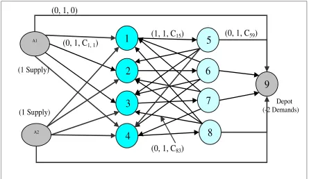
The problem for two vehicles and four jobs is demonstrated in Figure 2. In the figure the supply nodes are denoted by A1 and A2. Each of these nodes has a one unit supply. There is only a demand node in the MCF problem. This node has -2 units demand. The directed arcs from A1 and A2 to the demand node must be added to the network model. These arcs show that an AGV can remain idle without serving any job. Therefore, a cost of zero is assigned to these arcs. The lower bound, upper bound and cost of each arc are noted by the triplex

[Lower Bound, Upper Bound, Cost].

Solving the MCF problem generates 2 paths (the number of vehicles), each of which commences from a vehicle node and terminates at the demand node. Each path determines a job sequence of every vehicle. In figure 2, suppose that for some values of arc costs, the paths given by a solution are A1 1 5 4 8 9 and A2 2 6 3 7 9. This states that AGV 1 is assigned to serve jobs 1 and 4, and AGV 2 is assigned to serve jobs 2 and 3, respectively.

A1

1

5

2

6

3

7

4

8

9

(1, 1, C

15

)

(0, 1, C

59

)

(0, 1, C

83

)

(0, 1, C

1, 1

)

(0, 1, 0)

A2

(1 Supply)

(1 Supply)

Depot (-2 Demands)

Figure 2: The MCF model for 2 AGVs and four container jobs

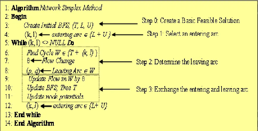
The NSA was chosen to tackle the MCF problem. The main reasons to choose NSA is that it is the fastest algorithm for solving the generalized network flow problem in practice . The algorithm in figure 3

Figure 3: The Network Simplex Algorithm (NSA)

Different strategies are available for finding an entering arc for the basic solution (see Step 1 in figure 3). These strategies are called pricing rules and the performance of the algorithm is affected by these strategies. The standard textbook and provided detailed accounts of the literature on those strategies. Some well-known strategies in NSA are the steepest edge scheme (by Goldfarb and Reid), the Mulvey’s list (by Mulvey), the block pricing scheme (by Grigoriadis), the BBG Queue pricing scheme (by Bradley, Brown and Graves), the clustering technique (by Eppstein), the multiple pricing schemes (by Lobel ]), the general pricing scheme (by Istvan ).

B. Simulated Annealing Method for the Multi-Load AGVs

The hardware technologies of AGVs are being improved to increase their capacity [18]. If the capacity of the AGVs increases, the problem defined in the section 2 is an NP-hard problem. This problem has a huge search space and must be tackled by one of the Meta-heuristics search methods. Although, Meta-heuristics usually also require relatively long computation times in order to provide good quality solutions, in some real-world applications meta-heuristics like Tabu Search and Simulated Annealing Method (SAM) might prove to be a good choice of method. This is due to the fact that these methods for the most part will be able to find a feasible solution within few seconds [25].

More research effort were observed recently on the SAM to improve their running times (see - ). This method could have significant impact on the speed up and the performance of the solutions We therefore restrict ourselves to SAM in this research.

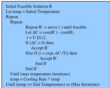
The SAM is analogous to the physical annealing process of obtaining a solid material in its ground state. A pseudo-code for the SAM is demonstrated in figure 4. For a description of the steps in this method and more details on parameters refer to [8] and [11].

Figure 4: A pseudo-code for SAM

C. The Hybrid of SAM and NSA for Heterogeneous AGVs

The NSA and SAM are solutions for the Single-Load and Multiple-Load AGVs problem, respectively. NSA provides the global optimum solution whereas SAM finds a local optimum for the problem. These two methods can be combined together to produce a hybrid method for Heterogeneous AGVs. Three following methods are considered to get an initial feasible solution for the SAM:

Deterministic Initial Feasible Solution: In this case, the tour length for each vehicle equals the total number of jobs divided by the total number of vehicles.

Random Initial Feasible Solution: Some random jobs can be chosen so those satisfy our feasibility constraints. This approach allows the process to begin at different neighborhoods.

Solutions from Network Simplex Algorithm: The

optimal solution from NSA for Single-Load AGVs provides an initial solution for SAM. Then, SAM can continue to find a better solution for Multi-Load AGVs.

The hybrid of SAM and NSA is based on the last option for the initial feasible solution. Regarding high performance of NSA, one can use the algorithm to produce an initial feasible solution for SAM.

5. EXPERIMENTAL RESULTS

To test the model and the algorithms, a hypothetical port was designed. The parameters in our experiment are the same as what we used in . The software was implemented in Borland C++ and then was run to solve several random problems on a Pentium 2.4 GHz PC with 1 GMB RAM. This section presents the experimental results for the problems of 50 AGVs and 7 quay cranes.

A. Running the Network Simplex Algorithm for Single-Load AGVs

As it was mentioned, the pricing rule or scheme in the NSA determines the speed of algorithm (see Step 1 in figure 3). Kelly and Neill implemented several pricing schemes and ran their software for different classes of minimum cost flow problems. In their results NSA with the Block Pricing scheme (NSAWBP) provided a better performance compared with others. The NSAWBP, therefore, was chosen. The CPU-Time required to solve the problems by the algorithm has been drawn in figure 5, according to the number of jobs. The power estimation for the curve has been also shown in the figure.

Figure 5: CPU-Time required to solve the problem for Single-Load AGVs by NSAWBP

Initial Feasible Solution R Let temp = Initial Temperature Repeat

Repeat

Repeat R` = move ( ) until feasible Let C = cost(R`) - cost(R) r = U [0,1]

If ( C < 0) then Accept R`

Else If (r < exp(- C /T)) then Accept R`

End If End If

Until (max temperature iterations) temp = Cooling Rate * temp

From the experiments, the following observations are gotten

Observation 1: NSAWBP is fast and efficient This observation shows that cycling is rare in this experience

Observation 2: NSWWBP is run in polynomial time to solve the problems, in practice In order to confirm this observation, the complexity of the algorithm was estimated. The result showed that the CPU-Time required to tackle the problem, is a function with degree 3 of the number of jobs in the problem .

Observation 3: Although NSAWBP is efficient and provides the optimal solution, it can only work on problems with certain limits in size The limitation is duo to available memory to put the MCF model into. Given |V| AGVs and n Container jobs, the number of arcs in the model is |V|×n+n×(n-1)+ |V|+2×n (see ). The largest problem, which has been solved by the software, was an MCF model consists of 11,058,350 arcs (|V|=50; n=3,300). This is the largest problem of Single-Load AGVs that was solved so far.

B. Running the Hybrid Method for Multi-Load AGVs

The values used for the parameters to run the hybrid method are shown in Table 1. These values have been

used in a research done by Galati et al. (1998) and it is shown that they led to significant results .

TABLE 1: SIMULATED ANNEALING PARAMETERS

Parameters Values Initial Temperature 1 End Temperature 4 Cooling Rate 0.999 Minimum String Limit 3 Iterations Per Temperature 1000 Total Iterations 30,000

Table 2 demonstrates number of container jobs and the values of objective function (traveling and waiting times of the vehicles as well as the lateness time to serve the jobs) by different options for the initial feasible solution of Simulated Annealing Method. The number of iterations in NSAWBP to solve the model for Single-Load AGVs is also shown in the table. Note that the number of iteration of running the NSA for the Single-Load AGVs (the 3rd column in Table 2) is not considerable compared with the number of iterations of Simulated Annealing Method for Dual-Load AGVs (the last row in Table 1). The percentages of increase in the objective function for the Deterministic Initial Feasible Solution and Random Initial Feasible compared with Initial Feasible Solution by NSAWBP are also calculated and put in the table.

TABLE 2

A

COMPARISON BETWEEN DIFFERENT OPTIONS FOR THE INITIAL POINTS OF

SAM

The Values of Objective Function by Simulated Annealing Method for Dual-Load AGVs Capacity along with the differences

Deterministic Initial Feasible Solution Constructive Random Initial Feasible Solution Problem Number

of Jobs

Number of Iterations in NSAWBP for

Single-Load AGVs

(1) Initial Feasible Solution by

NSAWBP

Objective Function

Percentage of Increase, compared with (1)

Objective Function

Percentage of Increase, compared with (1)

1 10 98 2452 11884093 99.98 2548 3.77

2 15 124 5444 61736113 99.99 5240 -3.89

3 20 160 7184 32438256 99.98 6617513 99.89

4 25 183 9905 190180985 99.99 3231285 99.69

5 30 243 1512972 258873766 99.42 2664134 43.21

6 35 299 926109 339936300 99.73 2617294 64.62

7 40 350 1520243 463498316 99.67 13250455 88.53

8 45 346 933279 678490771 99.86 8436397 88.94

9 50 560 1377087 29832 -4516.14 26769356 94.86

10 55 471 942830 3701579 74.53 27073631 96.52

11 60 541 1115226 30874299 96.39 27767825 95.98

12 65 613 5732181 55866349 89.74 21771211 73.67

13 70 681 3536178 142518848 97.52 32274173 89.04

14 75 632 2521881 192762995 98.69 68571331 96.32

15 80 827 4325901 298072454 98.55 100107503 95.68

16 85 842 6248466 392395471 98.41 83278606 92.50

17 90 1304 2514134 510167424 99.51 57437507 95.62

The value of objective function in Table 2 was analyzed statistically, according to 5% rejection on the ‘True Hypothesis’ (the two means are equal). Table 3 provides the test’s result along with the values of t-distribution for a particular degree of freedom. The student's t-test determines the means are significantly different at a 95% degree of confidence.

In this experiment, we got the following observations: Observation-4: If we choose some initial points for SAM by the Deterministic Initial Feasible Solution (DIFS) and Random Initial Feasible Solution (RIFS), then the objective function will become approximately 100% and 78% deteriorated respectively compared with an Initial Feasible Solution by NSAWBP (See the 6th and 8th columns in Table 2). Therefore, NSAWBP provides a significantly better initial point for SAM. It is due to the fact that NSA escapes from any local optimum and reaches to the global solution of the problem of Single-Load AGVs. Then, the hybrid method continues to find more optimal local solution for the problem of heterogeneous AGVs.

Observation-5: The Multi-Load AGVs problems have huge search space and few researches have been devoted on that. In a comparison, the size of problems solved for the Dual-Load AGVs here is very larger than on which focused (50 AGVs compared with 6 AGVs). This observation shows that the Multi-Load AGVs need more research and efficient algorithms in future.

TABLE 3

THE RESULT OF T-TEST FROM SAM WITH DIFFERENT OPTIONS FOR

INITIAL SOLUTION

Statistical Parameters

Initial solutions by NSAWBP and Deterministic initial

solution

Initial solutions by NSAWBP and Random initial

solution

Observations 18 18

T-Test (Paired Two Sample For Means )

-4.22193 -3.486049

Degree of Freedom 17 17

T Distribution 2.109819 2.1098185 6. CONCLUSION

In this paper, three solutions for the AGVs scheduling problem in container terminals are proposed. These solutions are Network Simplex Algorithm With Block Pricing (NSAWBP) for the Single-Load AGVs, Simulated Annealing Method (SAM) for Multi-Load AGVs and a hybrid of NSA and SAM for heterogeneous capacity of AGVs. The String Relocation as a neighborhood function and three options for the initial feasible solutions for the method (the solution from NSAWBP, deterministic and random job) were considered. Then, several the same random problems were generated and solved by the method. The experimental results showed a combination between NSAWBP and SAM provides a significantly better result when the capacity of the vehicles is increased to dual-load containers.

7. REFERENCES

Periodicals:

[1] E.P.K Tsang, “Scheduling techniques -- a comparative study”, British Telecom Technology Journal, Volume 13 (1), pp 16-28, Martlesham Heath, Ipswich, UK, 1995.

[2] B.J Wook and K.K Hwan,”A pooled dispatching strategy for automated guided vehicles in port container terminals”, International Journal of management science, Vol 6 (2), pp 47-60, 2000.

[3] Chiang, Wen-Chyuan and A.R Robert, “Simulated Annealing Metaheuristic for the Vehicle Routing Problem with Time Windows,” Annals of Operations Research, Vol. 63, pp 3-27, 1996. [4] M.D. Grigoriadis, ”An Efficient Implementation of the Network Simplex Method”, Mathematical Programming Study Vol. 26, pp 83-111, 1986.

[5] M Grunow, H.O Günther and M Lehmann, “Dispatching multi-load AGVs in highly automated seaport container terminals”, OR Spectrum, Volume 26 (2), pp 211-235, 2004.

[6] K.G.Murty, L.Jiyin, W Yat-Wah, C,Zhang C.L Maria, J. Tsang and L..Richard, “DSS (Decision Support System) for operations in a container terminal”. Decision Support System, Vol 39, pp 309-332., 2002.

Books:

[7] R.K.Ahuja, T.L.Magnanti and J.B.Orlin, “Network Flows: Theory, Algorithms and Applications”. Prentice Hall, 1993.

Technical Reports:

[8] Z.Czech and P Czarnas, “Parallel Simulated Annealing for the Vehicle Routing Problem with Time Windows. In Proceedings of 10th Euromicto Workshop on Parallel Distributed and Network-Based Processing, Canary Islands, Spain, pp 376-383, 2002. [9] Y.Huang and W.J.Hsu, “Two Equivalent Integer Programming

Models for Dispatching Vehicles at a Container Terminal”. CAIS, Technical Report 639798, School of Computer Engineering, Nan yang Technological University, Singapore, 2002.

[10] H.Sen, “Dynamic AGV-Container Job Deployment”. Technical Report, HPCES Programme, Singapore-MIT Alliance, 2001. [11] M.Galati, H.Geng, and T.Wu, “A Heuristic Approach For The

Vehicle Routing Problem Using Simulated Annealing”, Lehigh University, Technical Report IE316, 1998.

[12] Y. Cheng, H. Sen, K. Natarajan, T. Ceo, and K.Tan,"Dispatching automated guided vehicles in a container terminal", Technical Report, National University of Singapore, 2003.

Papers from Conference Proceedings (Published):

[13] S.H Chan, “Dynamic AGV-Container Job Deployment”, Master of Science, University of Singapore, 2001.

[14] H. Rashidi and E.P.K Tsang, "Applying the Extended Network Simplex Algorithm and a Greedy Search Method to Automated Guided Vehicle Scheduling", in Proceedings 2005, the 2nd

Multidisciplinary International Conference on Scheduling: Theory & Applications (MISTA), New York, Vol 2, pp 677-693. [15] T. Hasama, H. Kokubugata and H. Kawashima, “A Heuristic

Problem with Backhauls”, Proceeding of the 5th World Congress on Intelligent Transport Systems (ITS), Seoul, 1998.

[16] J.M. Patrick and P.M. Wagelmans, “Dynamic scheduling of handling equipment at automated container terminals”, Technical Report EI 2001-33, Erasmus University of Rotterdam, Econometric Institute, 2001.

[17] J.M. Patrick and P.M. Wagelmans, “Effective algorithms for integrated scheduling of handling equipment at automated container terminals”, Technical Report EI 2001-19, Erasmus University of Rotterdam, Econometric Institute, 2001.

[18] L. Qiu, W.J. Hsu, S.Y. Huang and H. Wang (2002), “Scheduling and Routing Algorithms for AGVs: a Survey”. International Journal of Production Research, Taylor & Francis Ltd, Vol. 40 (3), pp 745-760.

[19] L. Qiu, and W.J Hsu, “A bi-directional path layout for conflict-free routing of AGVs”. International Journal of Production Research, Volume 39 (10), pp 2177-2195, 2001.

[20] L. Qiu and W.J. Hsu, “Scheduling of AGVs in a mesh-like path topology”. Technical Report CAIS-TR-01-34, Centre for Advanced Information Systems, School of Computer Engineering, Nanyang Technological University, Singapore, 2001

[21] J. Böse, T. Reiners, D. Steenken, and S. Voß, ”Vehicle Dispatching at Seaport Container Terminals Using Evolutionary Algorithms”. Proceedings of the 33rd Annual Hawaii International Conference on System Sciences, IEEE, pp 1-10, 2000.

Dissertations:

[22] H. Rashidi, “Dynamic Scheduling of Automated Guided Vehicles in Container Terminals”, PhD Thesis, Department of Computer Science, University of Essex, 2006.

[23] D.J Kelly. and G.M. ONeill, "The Minimum Cost Flow Problem and The Network Simplex Solution Method", Master Degree Dissertation, University College, Dublin, 1993.

[24] C. Y Leong, "Simulation study of dynamic AGV-container job deployment scheme", Master of science, National University of Singapore, 2001