in the population sciences published by the Max Planck Institute for Demographic Research Konrad-Zuse Str. 1, D-18057 Rostock·GERMANY www.demographic-research.org
DEMOGRAPHIC RESEARCH
VOLUME 18, ARTICLE 7, PAGES 205-232
PUBLISHED 8 APRIL 2008
http://www.demographic-research.org/Volumes/Vol18/7/ DOI: 10.4054/DemRes.2008.18.7
Research Article
Does income inequality really influence
individ-ual mortality?
Results from a ’fixed-effects analysis’ where
constant unobserved municipality
characteris-tics are controlled
Øystein Kravdal
c
°2008 Kravdal.
1 Introduction 206
2 Possible mechanisms 208
2.1 Why should income inequality affect mortality? 208
2.2 Confounders 210
3 Data and Measures 211
3.1 Data 211
3.2 Computation of income variables 212
3.3 Regional variation 213
4 Models 214
4.1 Outline of the statistical approach 214
4.2 The simplest model, without municipality dummies 215
4.3 Model with municipality dummies 216
4.4 Remaining bias 218
4.5 Additional details about the variables 218
5 Results 219
6 Summary and Conclusion 226
7 Acknowledgements 227
References 228
Does income inequality really influence individual mortality?
Results from a ’fixed-effects analysis’ where constant unobserved
municipality characteristics are controlled
Øystein Kravdal1
Abstract
There is still much uncertainty about the impact of income inequality on health and mor-tality. Some studies have supported the original hypothesis about adverse effects, while others have shown no effects. One problem in these investigations is that there are many factors that may affect both income inequality and individual mortality but that cannot be adequately controlled for. The longitudinal Norwegian register data available for this study allowed municipality dummies to be included in the models to pick up time-invariant unobserved factors at that level. The results were compared with those from similar models without such dummies. The focus was on mortality in men and women aged 30-79 in the years 1980-2002, and the data included about 500000 deaths within 50 million person-years of exposure. While the models without municipality dummies suggested that income inequality in the municipality of residence, as measured by the Gini coefficient, had an adverse effect on mortality net of individual income, the results from the models that included such dummies were more mixed. Adverse effects appeared among the youngest, while among older men, there even seemed to be beneficial effects. In addition to illustrating the potential importance of controlling for unobserved factors by adding community dummies (doing a ’fixed-effects analysis’ according to common ter-minology in econometrics), the findings should add to the scepticism about the existence of harmful health effects of income inequality, at least in the Nordic context.
1Department of Economics, University of Oslo, Box 1095 Blindern, 0317 Oslo, Norway. Tel. (47)22855158.
1. Introduction
The idea that income inequality may weaken people’s health and increase mortality has attracted much interest in recent years (see e.g. reviews by Kawachi 2000; Wagstaff and van Doorslaer 2000; Lynch, Davey Smith, Harper et al. 2004; Wilkinson and Pickett, 2006). Some investigators have used an ecological approach to check whether societies (e.g. countries, states, municipalities) with large variation in income fare worse than oth-ers in terms of health and mortality, and many of these studies, but far from all, have concluded that there indeed seems to be such a relationship. A particularly robust pat-tern has been seen within the United States. However, a positive relationship between income inequality and mortality in an ecological analysis may simply reflect diminishing individual health returns to increasing individual income (see elaboration below). A more interesting question is whether individual health and mortality are adversely affected by the income inequality in the community net of individual income (see review of possible reasons below). This calls for a multilevel approach. Unfortunately, the answers to this question have been rather mixed. Whereas some studies have supported the hypothesis about adverse effects of income inequality - and especially American ones where in-equality has been measured at the state level - no effects, or in a few cases even beneficial effects, have shown up in other investigations.
When assessing the effect of income inequality, one should of course control for char-acteristics that are likely to influence both income inequality and health. One simple example of such a potential confounder is whether the place is urban or rural: urban so-cieties typically offer a diversity of jobs, and may therefore also produce large income differences, in addition to showing high mortality for many other reasons, at least in rich countries. While an urban-rural indicator may often be available to the researcher, there are a number of other socioeconomic, political, cultural or environmental factors that may also be confounders, and that may be difficult to measure, or at least not be available in the data at hand. Some of these unobserved factors may be approximately time-invariant, for example because they are somehow linked to the physical characteristics of the commu-nities, and these can be captured by including a 0/1-dummy variable for each community. In economic literature, such models are usually referred to as ’fixed-effects models’, and that label will be used occasionally in this paper also, although it has a broader meaning in much of the multilevel literature (see below).
aggre-gation than the community variables in focus (Mellor and Milyo 2002, 2003). However, in a recently published paper by Scheffler et al. (2007) on how psychological distress was affected by social capital measured in 58 U.S. Metropolitan Statistical Areas in three successive years, dummies representing that level of aggregation were included (and the authors pointed out that this was a novel approach). In this study, the effects became much stronger once the area dummies were included, but obviously one cannot generalize from that. The results may go in any direction.
When the intention is to assess how income inequality at a certain level of aggrega-tion affects mortality, the inclusion of dummies at that level is, of course, only possible if income inequality is observed two or more different times for each unit of aggrega-tion. (Otherwise, there would be no variation in income inequality net of the dummies.) Such data are scarce. However, the Norwegian register data available for this study pro-vided an excellent opportunity to estimate fixed-effects models of this type. They cov-ered the entire population, and included individual migration histories, as well as biogra-phies of, for example, individual education and income. In the migration histories, all municipalities in which a person had lived during the period under investigation were identified. The municipality, of which there are currently 431 in Norway, is the lowest political-administrative unit in the country (see details below). By aggregating up from the individual data, measures of income inequality and various other socio-economic char-acteristics of each municipality could be established for all relevant years. Thus, the data were, so to speak, longitudinal both at the individual and municipality level.
It is a common idea in this research area that income-inequality effects are most likely to show up at relatively high level of aggregation (e.g. Franzini et al. 2001), but it also seems plausible that the inequality at the municipality level may have some importance. One reasons is that Norwegian municipalities are responsible for some of the public health care and social support, though under strong national regulations. Little is known about the social and geographical extent of people’s comparisons with others, which is another factor that income inequality has been thought to operate through. Given modern commu-nication systems, people’s reference basis may often stretch far beyond the municipality, but it could also in many cases be restricted primarily to smaller neighbourhoods (or even socially defined subgroups of these neighbourhoods).
incomes than most other rich countries (e.g. United Nations 2006), but it is hard to be-lieve that their citizens do not react much like any other population to whatever inequality there is. The social and psychological mechanisms thought to be relevant for other rich countries are probably not completely irrelevant in the Nordic setting, although they may not necessarily produce a response of exactly the same strength, because of differences in political systems and ideological traditions. Results from earlier Nordic investigations, made at quite low levels of aggregation, have been somewhat mixed. On the one hand, income inequality was found to be unimportant both in a Swedish analysis of all-cause mortality based on about 40000 individuals living in 284 municipalities (Gerdtham and Johannesson 2004) and in Finnish studies on alcohol-related mortality and suicide in 84 ’functional regions’ (Blomgren et al. 2004; Martikainen et al. 2004). On the other hand, Dahl et al. (2006) reported a clear mortality-enhancing impact of income inequality when 88 ’economic regions’ in Norway were considered. In Denmark, Osler and her colleagues (2002, 2003) saw considerable variation in effects, for example across sexes and by level of aggregation (parish vs municipality), and even estimated some beneficial effects.
The paper is organized as follows: First, the existing ideas about why income inequal-ity may affect mortalinequal-ity are reviewed and discussed, and it is explained that certain factors may produce a spurious relationship between the two. The second step is to present the data that were used and describe the economic measures. Third, the models are specified. Because there is so little experience with this type of fixed-effects modelling in social epi-demiology, it is motivated and explained in some detail. Finally, the results are presented and conclusions are drawn.
2. Possible mechanisms
2.1 Why should income inequality affect mortality?
It is trivial that, all else equal, a person selected randomly from a municipality with large income inequality is more likely to have low or high income than a person selected ran-domly from a municipality with less inequality. Assuming that the positive health effect of high income is less pronounced than the corresponding negative health effect of low income, the person from the municipality with large income inequality will tend to have the highest mortality. In other words, if individual income is not included in the model, a mortality-enhancing effect of income inequality may be explained by diminishing health returns to individual income. However, it has also been argued that income inequality may affect a person’s mortality net of individual income (and net of average income, which may be linked with income inequality). Three main reasons have been suggested in the literature, and they are now briefly reviewed and discussed.
many people feel poor relative to others, which may produce a psychosocial stress that affects their health partly through psychoneuro-endocrine mechanisms and partly through health behaviour (e.g. Kawachi 2000; Wagstaff and van Doorslaer 2000; Lynch et al. 2004). This idea may be criticized for being too simplistic, however. For example, we do not know whether one is most harmed by seeing some who are very rich or many who are somewhat richer, and the extent to which any such effect can be buffered by being surrounded by people withlowerincomes. Anyway, the effect of the income distribution probably depends on where the person is located in this distribution.
A second main argument for an effect of income inequality (addressed for example by the authors referred to above) is that large differences between people with respect to incomes translate into differences in general opportunities and perhaps life styles. Further, awareness of all these differences, perhaps accompanied by feelings of inferiority (or superiority), may contribute to undermine ’social cohesion’, i.e. weaken people’s trust in each other and lower the chance that one may get assistance from others in case of health problems or more generally. However, there has not been overwhelming support for such an inverse relationship between income inequality and social cohesion, and it has not been consistently shown that social cohesion is important for health. Some researchers have argued that a high level of social cohesion improves the health, while others have seen no such effects (see e.g. Kawachi and Berkman 2000; Mohan, Twigg, Barnard and Jones 2005; Veenstra 2005) In fact, it has also been suggested that a cohesive community may contribute to overburden people with obligations (Martikainen, Kauppinen and Valkonen 2003), place problematic restrictions on individual freedom, or make life unnecessarily difficult for those who for some reason fall outside (Portes 1998).
A third suggested reason for a harmful effect of income inequality is that, although the relatively poor may want larger public investments in health and social services, the rich may favour a lower tax level and have a dominant voice (see once again the same references). This argument may have modest relevance for the country analysed here, however. The quality of some important health and social services in Norway does de-pend on decisions taken locally, in addition to national regulations and national and local economic resources, but these decisions are in principle rooted in local elections, which (especially given the relatively high participation rates) should reflect the interests of rich and poor alike.
or that a high prevalence of health problems might reduce the access to health services for other people (i.e. a ’crowding out’ argument)?
Finally, given the average income, a high level of inequality will increase the tax revenues in a country with progressive taxation, such as Norway. This could, for example, contribute to a higher quality of the health services.
To summarize, there are some arguments for adverse effects of income inequality, most of them apparently quite widely accepted. However, they all have their weaknesses, and it is possible to argue for the opposite as well, i.e. that large inequality may promote betterhealth. There is even a little empirical support for the latter: Beneficial effects have shown up in a few multilevel studies, at least for certain sub-populations and without control for some variables that have a particularly ambiguous causal position (Mellor and Milyo 2003; Osler, Christensen, Due et al. 2003; Wen, Browning and Cagney 2003). The authors have not given these negative findings much attention, though, and have not felt tempted to offer any causal interpretations.
2.2 Confounders
A statistical association between income inequality and mortality may not necessarily reflect only causal effects such as those just mentioned. It may also to some extent be a result of factors affecting both income inequality and mortality.
Generally, the income inequality in a community at any given time depends on the variations in the types of jobs, in the citizens’ skills and interest in and need for work, and in the income returns to given inputs in these jobs. These factors are in turn determined partly by (approximately) time-invariant environmental and cultural factors. For example, in a fairly isolated small coastal community, job creation may to a large extent hinge on the marine resources. If everyone is either involved directly in the fishing or the fishing industry or provides various services to the modestly paid people in this sector, the in-come distribution will be narrow. Similarly, small-scale agriculture may be the dominant activity in certain rural areas with a topography that is not suitable for large farms, while small places close to waterfalls and a good harbour may specialize in energy-intensive manufacturing. In such communities, there may also be an advanced service sector that offers higher wages, but that may depend partly on the distance to schools and whether better-educated people from other areas for some reason are attracted to this place. In cities, one may expect more variation in jobs and incomes (e.g., Nielsen and Alderson 1997): Some may work in factories, while others may be involved in low-paid service activities or have well-paid jobs in the public administration or the (typically more remu-nerative) private service sector. Getting work in the advanced service sector is probably most likely in cities that are very large or serve as some kind of regional centre.
volatile forces with immediate effects. For example, shifts in international prices or changing consumer tastes may rather quickly reduce the demand for some of the goods or services produced in a certain community, which may lower the earnings of those in-volved in this particular work without having much impact on others. Another example may be that new laws or regulations, at the local or national level, make some already profitable activities in some communities even more profitable, or politicians with less in-terest in supporting companies with problems may come into power so that more people become unemployed.
Some of the factors that affect the income inequality may also have an impact on mortality through completely different channels. For example, a rural environment may encourage health-promoting physical activity, and living in a fishing community may af-fect the diet in a positive way. In cities, the short distance to a hospital is a potential advantage, but on the other hand, the high population density may increase the incidence of respiratory diseases. Besides, high population density may (not only because of the possibly high income inequality) contribute to a diversity of lifestyles and a weakening of social control that may have good as well as bad effects. Further, fundamental changes in political attitudes may affect not only the income distribution, but also the quality of health and social services, the efforts to control drug abuse, or other factors of importance for people’s health.
3. Data and Measures
3.1 Data
The data used in this analysis were taken from population censuses and various national population registers, and included all men and women who had lived in Norway and were of age 30-79 some time during 1980-2002. Similar data have been used in several previous studies (e.g. Kravdal, 1995, 2000, 2007). For each person, the data included information about date of death, cause of death, the highest educational level attained as of 1 October each year since 1980 and for some earlier years (based on school reporting and earlier censuses), and gross annual labour income reported to the tax authorities each year since 1968 (converted to 1000 Norwegian Kroner (NOK) in 1998 prices, by means of the consumer price index). A person’s purchasing power does not depend only on gross labour incomes, but also on the income of the partner (if any), the number of persons in the household, accumulated wealth, taxes, public transfers, and (especially for the elderly) pensions. However, no attempt was made to gather such data.
These codes were not equal to the real municipality numbers, so municipalities could not be identified. However, municipality variables could be constructed by aggregating over the individual data.
There were 433 municipalities in these data, but because of a few recent border changes, the current number is 431. The population is very unevenly distributed over these municipalities. Oslo, the capital, has about half a million inhabitants, and there are 4 other large urban municipalities with a population of 100000 - 250000. Among the other municipalities, the average population size is about 7000, with a variation from 200 to 75000. In one set of models, the 19 counties (which were identified) were used instead as the aggregate units.
3.2 Computation of income variables
The definition of the Gini coefficient can be found in any introductory textbook in eco-nomics. To build up the definition, let us start with the Lorenz curve for income distri-bution in a certain population. Each point(r, s)on the Lorenz curve tells us how large proportionsof the total income that is earned by the proportionrwho earn least. If every-one earns the same, the Lorenz curve is a 45-degree diagonal(s=r). In contrast, if only one person earns money, the curve is 0 up tor= 1, where it bounces up to 1. Denoting the area under the Lorenz curve asL, the Gini coefficientGis defined as the area between the 45-degree diagonal and the Lorenz curve, divided by the area below the diagonal, i.e.
G= (0.5−L)/0.5 = 1−2L. Thus it is 0 in the first of the extreme examples given (whereL= 0.5) and 1 in the second (whereL= 0).
In this analysis, a continuous version of the Gini coefficient was calculated (rather than grouping first the persons into, for example, the 10% earning most, the 10% earning second most etc.). More specifically, theN individuals at age 30-69 in a municipality were sorted by their annual income, in ascending order. Denoting the sum of the incomes for the firstipersons asY(i), and settingY(0) = 0, the Gini coefficient was calculated as
G= 1− P
iY(i) +Y(i−1)
N·Y(N) ,
where the summation runs fromi= 1toi=N.
The age group 30-69 was chosen because at least most of the men work at that age. Also an average-income variable was calculated for this age group. Unless otherwise stated, both sexes were included when average income was computed, while women were excluded in the computation of the Gini coefficient. However, alternatives were tried (see elaboration below)2.
3.3 Regional variation
The physical environment in Norway is very diverse. There are, for example, densely populated urban areas as well as small coastal communities and a great variety of inland rural settlements. The travel time to a large city is long for many people, partly because of deep fjords or high mountains. This variety creates differences in economic activity and lifestyles, and even with a political ideology that places emphasis on equality of opportunities (e.g. Kautto, Heikkilä, Hvinden and Marklund 1999), it is hard to avoid a certain variation in incomes and in the access to health and other services. For example, the mean of the average income over the 23 years under study was twice as high in the richest municipalities as in the poorest (the national mean was 126000 NOK and the standard deviation of the municipality 23-year means was 27000 NOK).
There is also substantial variation in income inequality. The minimum and maximum values of the Gini coefficient were 0.23 and 0.51, the standard deviation was 0.05, and the mean was 0.37. 23% of the variance waswithinmunicipalities. To elaborate on the latter component, which is essential when municipality dummies are included, the within-municipality increase in the Gini coefficient was 0.0014 per year as a national average if we assume a linear trend. This corresponds to 0.030 over the 23-year period. The standard deviation (across municipalities) of the 23-year change was 0.046, the minimum value was -0.16, and the maximum value was 0.14.
A municipality-level regression model revealed that the Gini coefficient in the 5 largest municipalities was relatively large. Among other municipalities, however, there was no relationship between income inequality and population size. Thus, there was quite modest support in the Norwegian data for the idea mentioned earlier that urban areas, which tend to be found in municipalities with large population size, may have large income
ity. Further, there was a quite clear negative relationship between the Gini coefficient and the average income (the correlation coefficient was -0.6). The highest levels were found in Northern Norway and the lowest in Western and Central Norway. With these data, the factors that were responsible for the regional pattern could not be identified.
Finally, it might be noted that regional differences in mortality do appear in Norway, for example at the county level: Men’s life expectancy at birth currently ranges from more than 78 years in some counties in Western Norway to less than 75 years in the northern county of Finnmark (Statistics Norway 2007), with the corresponding figures for women being 83 and 81 years. These differences may reflect variations in the economic situation as well as many other factors.
4. Models
4.1 Outline of the statistical approach
Discrete-time hazard regression was chosen as the statistical tool (using the Proc Logistic module in the SAS software), and the models were estimated separately for men and women and for the five age groups 30-39, 40-49, 50-59, 60-69, and 70-79. This was because of the large size of the data. In all groups combined, the total exposure time was about 50 million person-years (and there were about 500000 deaths).
Using women of age 70-79 as an example, the follow-up was from January the year the woman turned 70, but not earlier than 1980. End of follow-up was at the time of death or emigration, the end of 2002, or the end of the year when the woman turned 79, whatever came first. Each person contributed a series of 12-month observations. (These intervals were sufficiently short, because a length of 6 months gave the same results.) All individual variables were time-varying and referred to the situation at the start of the 12-month observation interval or earlier. The municipality variables referred to the situation in the observation interval in the municipality in which the person lived at the beginning of that interval.
the age and sex variations in the relationship between income inequality and health (e.g. Lynch et al. 2004)3.
Some attention was also paid to the possibility that the effect of income inequality may depend on the person’s own individual socio-economic resources (for which one argument was given earlier). The findings from earlier studies have been mixed, but point in the direction of most harmful effects among people who themselves have little resources (Dahl et al. 2006). In addition, a few cause-specific models were estimated, since some of the suggested mechanisms may be more relevant for some causes of death than for others. For example, there has been particular support for an adverse effect of income inequality in studies focusing on homicide or other violent deaths (e.g. Lynch et al. 2004).
4.2 The simplest model, without municipality dummies
The models were of two types. One was the following:
log pijt
1−pijt =γ0+γ1Xijt+γ2Zjt+γ3Tt, (1)
wherepijtis the probability that personiin municipalityjobserved in the time intervalt
dies within that interval,γ0is a constant term,Xijtis a vector of individual characteristics
(income, education, and age), Zjt is a vector of municipality characteristics (average
income, income inequality and in some models average education), andγ1andγ2are the
corresponding effect vectors. All the municipality variables were time-varying, though it would of course be possible to include also time-invariant ones.Ttis a vector of dummies
representing one-year periods (one dummy for each year except one arbitrarily chosen reference year). It was included to pick up other and national-level factors that may change over time and influence mortality, such as the medical treatment technology. If there is no such period variable in the model, the estimated effect of income inequality will to some extent reflect the correlation between the overall mortality trend due to these other general factors and the trend in income inequality.
It has become very common in multilevel analysis to add a time-invariant random term to the intercept. The term is typically assumed to be drawn independently for each
3For example, Lobmayer and Wilkinson (2002) (in an ecological analysis) and Backlund et al. (2007)
unit of aggregation, with 0 mean and a variance to be estimated, and to be uncorrelated with the observed co-variates. In our case, the model would then be:
log pijt
1−pijt =γ0+γ1Xijt+γ2Zjt+γ3Tt+Dj, (2)
whereDj is this random term. (In principle, municipality-level random terms may also
be added to the effect parameters, or the term may be period-specific.)
The motive for this model specification is that there are certain characteristics of a municipality that affect everyone, but that are not captured by the included variables. This has the implication that observations from one municipality, so to speak, should not be reckoned as independent when making inferences about the municipality-level effects. Put differently, without taking into account that people have something unobserved in common, one would overstate the significance of the municipality effects. Accordingly, what one actually finds is that inclusion of this type of random term increases the standard errors of the municipality-level effects. The point estimates, however, remain essentially unchanged. For further details, see for example Goldstein (2003).
Such models with a random term are hard to estimate when the data material is as large as in this analysis. For example, neither aML nor MLwiN can handle so many observa-tions (per higher-level unit). Experiments with the NLMIXED procedure in SAS were not successful either. Hundreds of hours of computer time were needed for convergence, even with simplified versions of the models, and the results were suspicious.
4.3 Model with municipality dummies
In this analysis, municipality dummies were added instead of a random term. Also these dummies represent unobserved time-invariant municipality factors, but there is no as-sumption that these community factors are uncorrelated with the other regressors. In other words, one takes into account that there may be some constant characteristics that for example make income inequality high and also produce a high mortality. If inclu-sion of the municipality dummies changes the estimate of the income-inequality effect, it would mean that the time-invariant unobserved municipality factorsarecorrelated with income inequality, and that a model with a random term therefore would be inappropriate, as would of course also the simpler model without such a term.
More specifically, models of this form were estimated:
log pijt 1−pijt
=γ0+γ1Xijt+γ2Zjt+γ3Tt+γ4Fj, (3)
where the vectorFj consists of dummies for each of the 433 municipalities except one
In this case, effects of municipality variables can only be estimated if there are multiple measurements of these variables (i.e.Zjtmust be time-varying, as here).
It is common in econometric literature to denote the municipality dummies or the corresponding coefficients as ’fixed effects’, and the model as a ’fixed-effects model’. In contrast, the model presented earlier, where the unobserved factors are represented by a random term, is denoted as a ’random-effects model’. However, according to common terminology in much of the other statistical literature, all the terms on the right-hand side of (3) would be ’fixed effects’, not only the last one, and the model (2) including also a random term would be a ’mixed model’. In this paper, ’fixed effects model’ is used occasionally as a label for the model with municipality dummies.
Inclusion of municipality dummies means that the relationship between the overall levels (time averages) of income inequality in the municipalities and the respective mor-tality levels is ignored, because it is suspected to be too influenced by constant common municipality-level determinants. Instead, the effect of income inequality is identified ex-clusively from the relationship between time changes in income inequality and in mor-tality within each municipality. To get some intuitive understanding of the model, let us for a moment disregard the effects of period and consider only persons with certain given individual characteristics, and only observation periods and municipalities with a certain given level of the other municipality factors. If we assume a positive effect of income inequality, the model would then predict that, within each municipality, mortality is high among observations made when inequality is high and low among observations made when inequality is low. Put differently, if persons living in a certain municipality in a period when income inequality is high have higher mortality than persons living there when income inequality is low, that municipality contributes to a positive estimate of the income-inequality effect (see Appendix for elaboration). It is more complicated when the time dummies are included. In that case, we may say that a positive (negative) effect is estimated in the fixed-effects approach if municipalities with relatively large increases in income inequality have relatively large (small) increases in mortality, at given levels of the other covariates.
The fixed-effects approach has obvious disadvantages. Adding so many parameters places large demands on the computer, and the standard errors of the other municipality-level variables become much larger. Further, some of the Norwegian municipalities are very small, which produces large standard errors of the corresponding coefficients (γ4)4.
Because the municipalities cannot be identified either, the coefficients are not shown. In some models, the 100 smallest municipalities were left out. This gave the same patterns in the inequality-effect estimates (not shown). Exclusion of the 5 largest municipalities
4All the municipality coefficients were between -0.7 and 0.4 for women and men aged 70-79, and about 1/4
resulted in a negative effect for women aged 70-89 that was not seen in other models, but otherwise left little imprint on the estimates (not shown).
4.4 Remaining bias
Ideally, one would prefer to estimate a causal effect of income inequality, which we may think of as telling us about the change in mortality that occurs if a person with certain characteristics is moved from one community to another that is similar except for an-other level of income inequality, or if a person with certain characteristics experiences an immediate increase in income inequality in the municipality of residence while all other municipality characteristics remain unchanged. However, there are two main reasons why even the fixed-effects approach may not give us such an estimate. One reason is that there may be unobserved time-varying municipality factors. If, say, a large increase in mor-tality is seen in communities with large growth in income inequality, given individual and other municipality characteristics, some or all of this might in principle be due to common unobserved time-varying determinants, for example local policies. The munici-pality dummies do not pick up these unobservedtime-varyingfactors, only those that are time-invariant.
The other problem that remains with the fixed-effects approach is unobserved individual differentials related to selective migration. To illustrate, let us for simplicity ignore the time variable and the other municipality variables, and consider persons with certain given observed individual characteristics. Some may be observed in a municipality when the income inequality is low and others may be observed in the same municipality when the income inequality is high. In principle, the latter may to a larger extent than the former for example have some unobserved characteristics that produce high mortality - characteris-tics that are not a consequence of the high income inequality, which would be a causal pathway that we might not necessarily want to leave out, but characteristics that have increased their chance of living in that municipality at that time. Put differently, high in-come inequality (or community characteristics associated with it) may make people with certain unobserved characteristics move to or remain in the municipality, and these char-acteristics may also influence mortality. This is not a mechanism one would consider part of the causal effect.
4.5 Additional details about the variables
the economic situation) that are also the reason for the death. While not a perfect solution, it would at least help to lag the income variable more years, and that also seems a good strategy because any causal effect of income may need some time to be felt. Given also the substantialvariationsin income over time for some persons, the individual average income over the years 6-10 before the observation interval was used as the individual in-come variable. Years with missing inin-come (because the person did not live in the country) were ignored when calculating this average. If there was no income information for any of the 5 years, the income variable was set to 0 (any number would do) and a missing-income variable was set to 1 (otherwise 0). There were about 1% such missing-missing-income observations.
Because there is no similar endogeneity problem at the aggregate level, income in-equality and average income can be based on income data for the observation inter-val. However, some models with lagged income-inequality and average-income variables were estimated, because this makes good sense theoretically: While it is possible, for example, that other people’s affluence may cause a quite immediate feeling of inferior-ity with a quick influence on for example the suicide risk, effects operating through the feeling of solidarity in society, and thereby the quality of social networks, may not ma-terialize so quickly (see Blakely, Kennedy, Glass and Kawachi (2000) and Mellor and Milyo (2003), who found sharper effects of a lagged variable than when current income inequality was considered.) To simplify a little, using a lag of for example 10 years in a fixed-effects approach means that the trend in mortality over a certain period is compared with the trend in income inequality 10 years earlier, rather than with the trend over the same period (which may be different).
There has been a discussion in the literature about the inclusion of education in mod-els used to assess effects of income inequality (e.g. Lynch et al. 2004). On the one hand, a person’s current educational level is a very important determinant of that person’s income, and, similarly, community education has a bearing on the general level and distribution of income. On the other hand, current education may also be aresultof the community’s investments in education some years back, which in turn is linked with the degree of in-come inequality at that time. In this study, individual education was included in all models (grouped into 4 levels and with a special indicator for the 2% with missing education), while average education (over ages 30-69) was included only in some models.
5. Results
munic-ipality dummies. This is seen in Table 1, where all effect estimates for women at age 70-79 are shown as an example, and in Table 2, where only the effects of the Gini co-efficients are shown. There was a clear age pattern: The higher the age, the weaker the income-inequality effect.
All these effects of income inequality in the simplest models were significant. We do not know how large the standard errors would have been if it had been possible to follow the common strategy and add a municipality-level random term, but it is worth noting that even if they were twice as large as in the models with municipality dummies, the effects would still be significant.
When the municipality dummies were added, the model fit improved significantly (the changes in−2log Lwere between 550 and 2300, which correspond to significance levels below 0.01; values only shown in Table 1). On the whole, the income-inequality effects became less positive, but there were some differences across age and sex (Table 2). The effects for men were only significantly adverse at age 30-39, and there were indication also at age 40-49, while the effects at higher ages were beneficial, or (for age 50-59) there was at least an indication in that direction. Among women, there were no significant effects at any age5.
Note that it would not be appropriate in this situation to just include a random term to pick up unobserved municipality characteristics, which is typically done in multilevel epi-demiological research these days. That approach is based on a no-correlation assumption that is clearly violated.
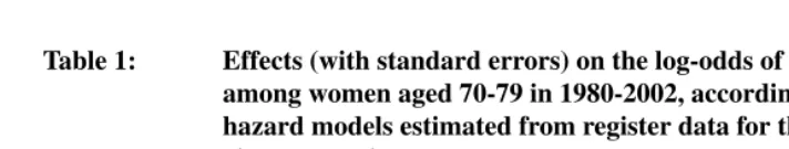
Table 1: Effects (with standard errors) on the log-odds of all-cause mortality among women aged 70-79 in 1980-2002, according to discrete-time hazard models estimated from register data for the entire Norwe-gian population
Model without Model with
municipality dummies municipality dummies (’Fixed-effects model’)
Gini coefficient in the municipality 1.223 **** (0.079) 0.271 (0.178)
Average income in the municipality (in 1000 NOK) 0.0015 **** (0.0001) 0.0007 (0.0006)
Individual income (in 1000 NOK) −0.0038 **** (0.0001)−0.0038 **** (0.0001)
5It might also be noted from Table 1 that the mortality-enhancingeffect of high average income seen in the
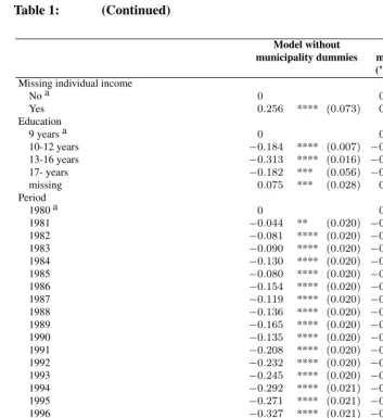
Table 1: (Continued)
Model without Model with
municipality dummies municipality dummies (’Fixed-effects model’)
Missing individual income
No a 0 0
Yes 0.256 **** (0.073) 0.259 ** (0.073)
Education
9 years a 0 0
10-12 years −0.184 **** (0.007) −0.179 **** (0.007)
13-16 years −0.313 **** (0.016) −0.308 **** (0.016)
17- years −0.182 *** (0.056) −0.178 *** (0.006)
missing 0.075 *** (0.028) 0.075 *** (0.028)
Period
1980 a 0 0
1981 −0.044 ** (0.020) −0.040 ** (0.020)
1982 −0.081 **** (0.020) −0.069 **** (0.020)
1983 −0.090 **** (0.020) −0.071 **** (0.020)
1984 −0.130 **** (0.020) −0.105 **** (0.020)
1985 −0.080 **** (0.020) −0.051 ** (0.020)
1986 −0.154 **** (0.020) −0.118 **** (0.022)
1987 −0.119 **** (0.020) −0.080 **** (0.022)
1988 −0.136 **** (0.020) −0.089 **** (0.023)
1989 −0.165 **** (0.020) −0.114 **** (0.023)
1990 −0.135 **** (0.020) −0.075 *** (0.024)
1991 −0.208 **** (0.020) −0.140 **** (0.025)
1992 −0.232 **** (0.020) −0.158 **** (0.026)
1993 −0.245 **** (0.020) −0.152 **** (0.029)
1994 −0.292 **** (0.021) −0.204 **** (0.029)
1995 −0.271 **** (0.021) −0.185 **** (0.030)
1996 −0.327 **** (0.021) −0.241 **** (0.032)
1997 −0.326 **** (0.021) −0.236 **** (0.035)
1998 −0.353 **** (0.022) −0.261 **** (0.039)
1999 −0.380 **** (0.022) −0.281 **** (0.042)
2000 −0.408 **** (0.022) −0.304 **** (0.044)
2001 −0.432 **** (0.023) −0.320 **** (0.046)
2002 −0.410 **** (0.023) −0.301 **** (0.051)
Age (years) 0.105 **** (0.001) 0.105 **** (0.001)
Municipality fixed effects Yes
−2Log L 1064731 1063424
a Reference category
Table 2: Effects (with standard errors) of the Gini coefficient on the log-odds of all-cause mortality among men and women aged 30-79 in 1980-2002, according to discrete-time hazard models estimated from reg-ister data for the entire Norwegian population a
Model without Model with
municipality dummies municipality dummies (’Fixed-effects model’)
MEN
30-39 3.109 **** (0.260) 2.562 **** (0.636)
40-49 2.356 **** (0.198) 0.938 * (0.479)
50-59 1.852 **** (0.137) −0.558 * (0.315)
60-69 1.445 **** (0.091) −0.581 *** (0.208)
70-79 1.126 **** (0.068) −1.605 **** (0.152)
WOMEN
30-39 3.648 **** (0.399) 0.205 (0.968)
40-49 3.041 **** (0.275) 0.152 (0.682)
50-59 2.218 **** (0.191) 0.046 (0.443)
60-69 2.071 **** (0.126) −0.089 (0.288)
70-79 1.223 **** (0.079) 0.271 (0.178)
a Age, calendar year , individual income, individual education, and average income were also included. *p <0.10; **p <0.05; ***p <0.01; ****p <0.001
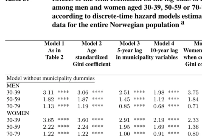
As a robustness check, a series of alternative models were estimated, though only for men and women aged 30-39, 50-59 and 70-79 because of the long computer time. More precisely, the following was done (only estimates from the models with municipality dummies are referred here; estimates from simplest models, which were all positive, can be seen in the table):
1. Some other age restrictions (30-59, 30-64) were chosen when calculating the Gini coefficient. This gave the same pattern in the estimates (not shown).
2. Age standardization was tried when computing the Gini coefficient, because it might otherwise pick up the age structure (e.g. large inequality may be a result of a large proportion relatively old or young), which in turn may be linked to mor-tality in a complex manner. Fortunately, this also gave the same results, except that the effect for women of age 70-79 attained significance at the 10% level (Model 2, Table 3).
municipality. With a 5-year lag, the results were very similar, but the point estimate for women aged 30-39 was more positive, and a more clearly significant beneficial effect appeared for men aged 50-59 (Model 3, Table 3). With a 10-year lag, this adverse effect for the youngest women turned significant, while the adverse effect for the youngest men was now only significant at the 10% level (Model 4, Table 3). Also inclusion of average income and income inequality 5 or 10 years earlier in the municipality where the person lived at the start of the observation interval (rather than 5 or 10 years earlier), gave very similar results (not shown). The data did not allow experimentation with lags longer than 10 years.
4. Women were included when calculating the Gini coefficient. Once again, the same pattern showed up in the mortality effect estimates, though there was a clearer indi-cation of an adverse effect among women aged 70-79 and the effect for men aged 50-59 was more strongly significant (Model 5, Table 3).
5. Average education at age 30-69 was added to the model, which had no impact on the estimated effects of the Gini coefficient (Model 6, Table 3). (According to the model with municipality dummies, a high average education at age 30-69 reduced mortality significantly among women at age 50-59. Otherwise, this variable had no effect.)
6. The average income among men was included, rather than that for both sexes pooled. This gave the same pattern in the estimates (not shown).
7. Generally, inclusion of individual income makes the effects of inequality less pos-itive or more negative, but the differences are rather small (not shown). To see whether a better control for individual income would be important, a grouped vari-able with 13 categories, including one for 0 income, was tried as an alternative. This gave very similar results (not shown). Shorter lags were also tried. For example, the inclusion of income 1-5 years before, rather than 6-10 years before, led to nearly the same estimates (not shown). For men and women at age 70-79, an additional model included average annual income during an earlier period, age 50-59, when at least the men were very likely to have worked (excluding years before 1968, for which the income is not known, or any year abroad). Earlier labour incomes may themselves be important, in addition to determining the level of the retirement pen-sions. A strongly significant beneficial effect of high income inequality was still seen among men, while a harmful effect showed up for women, now significant at the 5% level (not shown).
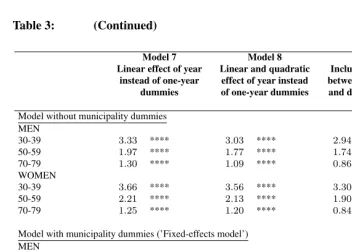
tried, as a simple robustness check. First, a linear trend was assumed by putting in year instead of the one-year dummies. That gave similar results, except that a significantly adverse effect appeared for women aged 70-79 (Model 7, Table 3). Second, a quadratic term for year was added, which made the effect for this group non-significant again (Model 8, Table 3). Third, the one-year period effects were al-lowed to vary across main regions (Eastern, Southern, Western, Central and North-ern Norway) by introducing period-region interactions. Also this specification led to similar results (Model 9, Table 3). (Obviously, if the time trend had been al-lowed to differ freely across municipalities, the model would not be identified, as all within-municipality mortality variation could be explained by the time trend.)
Table 3: Effects of the Gini coefficient on the log-odds of all-cause mortality among men and women aged 30-39, 50-59 or 70-79 in 1980-2002, according to discrete-time hazard models estimated from register data for the entire Norwegian population a
Model 1 Model 2 Model 3 Model 4 Model 5 Model 6
As in Age 5-year lag 10-year lag Women included Average Table 2 standardized in municipality variables when computing education
Gini coefficient Gini coefficient 30-69 also
included
Model without municipality dummies MEN
30-39 3.11 **** 3.06 **** 2.51 **** 1.98 **** 3.75 **** 3.01 **** 50-59 1.82 **** 1.87 **** 1.45 **** 1.12 **** 1.84 **** 1.79 **** 70-79 1.13 **** 1.19 **** 0.85 **** 0.68 **** 0.71 **** 1.06 **** WOMEN
30-39 3.65 **** 3.60 **** 2.91 **** 2.19 **** 2.33 **** 3.43 **** 50-59 2.22 **** 2.24 **** 1.95 **** 1.69 **** 1.36 **** 2.17 **** 70-79 1.22 **** 1.22 **** 1.00 **** 0.91 **** 0.80 **** 1.24 ****
Model with municipality dummies (’Fixed-effects model’) MEN
30-39 2.56 **** 2.67 **** 2.27 **** 0.90 * 3.07 **** 2.65 **** 50-59 −0.56 * −0.52 * −1.10 **** −1.07 **** −1.02 *** −0.60 * 70-79 −1.61 **** −1.54 **** −1.52 **** −1.50 **** −1.85 **** −1.60 **** WOMEN
30-39 0.21 0.27 1.21 1.62 **** 0.19 0.08
50-59 0.05 −0.04 0.01 −0.12 0.05 −0.11
Table 3: (Continued)
Model 7 Model 8 Model 9
Linear effect of year Linear and quadratic Included also interactions instead of one-year effect of year instead between one-year dummies
dummies of one-year dummies and dummies for five main regions
Model without municipality dummies MEN
30-39 3.33 **** 3.03 **** 2.94 ****
50-59 1.97 **** 1.77 **** 1.74 ****
70-79 1.30 **** 1.09 **** 0.86 ****
WOMEN
30-39 3.66 **** 3.56 **** 3.30 ****
50-59 2.21 **** 2.13 **** 1.90 ****
70-79 1.25 **** 1.20 **** 0.84 ****
Model with municipality dummies (’Fixed-effects model’) MEN
30-39 2.44 **** 1.84 **** 1.97 ***
50-59 −0.35 −0.90 **** −0.49
70-79 −1.17 **** −1.60 **** −1.83 **** WOMEN
30-39 0.18 −0.06 −0.58
50-59 0.06 −0.24 −0.02
70-79 0.44 *** 0.27 −0.06
a Age, calendar year , individual income, individual education, and average income were also included. *p <0.10; **p <0.05; ***p <0.01; ****p <0.001
To see whether effects of income inequality perhaps were more adverse among the socio-economically least advantaged, models were estimated separately for i) those with only compulsory education (about half in the oldest age groups and 20% in the youngest) and ii) for men aged 50-59 or 60-69 with an income below the average for men aged 30-69 in the municipality that year (since individual income refers to the situation 6-10 years earlier, and the general annual growth in incomes is only a few percent, the current average for the 30-69 age group would be a reasonable reference). It turned out that large inequality was not particularly harmful for any of these groups. In fact, the estimates were very similar to those for all persons in the respective age groups (not shown).
(not shown). The only difference worth mentioning is that, when the municipality dum-mies were included, the effect among women at age 70-79 was more markedly adverse (point estimate 0.77, significance level <0.01).
Finally, models were estimated for a few specific causes of death for which earlier studies have suggested particularly adverse effects of income inequality, or of low so-cial cohesion (see also Martikainen et al. 2003): Alcohol related deaths, suicide, and all violent deaths pooled. There were no harmful effects in any of these models when mu-nicipality dummies were included (not shown). Homicide was not considered separately, since there were only about 50 such deaths in the country each year.
6. Summary and Conclusion
Norway is a more egalitarian country than most others, and a low level of aggregation was chosen in this analysis. Nevertheless, significantly adverse effects of income inequality (net of the persons’ individual income) were estimated for all age groups and both sexes in the model without municipality dummies. The effects were sharpest among the youngest. Perhaps inferiority is less intensely felt at the higher ages, or perhaps the psychosocial and other factors potentially influenced by income inequality have more effect on the causes of death occurring relatively frequently at low ages, such as violent deaths. In that case, however, one would expect stronger effects on these causes of death in the models estimated for the older men and women, which did not appear.
It is interesting to see that the adverse effects of income inequality among the youngest survived the addition of municipality dummies (significant for women aged 30-39 when the income-inequality variable was lagged 10 years, and for men when there was no lag). Besides, there were indications in the same direction for men in their 40s, and adverse effects appeared for 70-79 year old women with certain model specifications. Apart from that, this fixed-effects approach did not support the idea that high income inequality is harmful, and among older men (and among older women when the 5 largest municipalities were left out), there even seemed to bebeneficialeffects.
Non-positive effects are not theoretically implausible. As mentioned earlier, the com-mon ideas about causal mechanisms can be criticised. For example, can we be so sure that income inequality really undermines social cohesion substantially, or that it is responsible for generally stressful feelings of relative deprivation? Does weakened social cohesion really exert the allegedly harmful health effect? Is it actually the case that rich people can block poorer people’s interest in improving social services? In fact, one may even find arguments for beneficial effects. However, it is not easy to understand why the adverse as well as the beneficial effects should be particularly pronounced for men.
the municipality dummies only pick up the constant unobserved factors that may have a bearing on both income inequality and individual mortality, such as for example environ-mental characteristics. The estimates may in principle be biased because of unobserved time-varyingcommunity factors and selective migration. Further, the measurement of income is not ideal. It is the individual gross labour income that is available rather than household disposable income. Control for individual income appeared not to be very im-portant, so the key issue is probably whether a Gini coefficient computed from individual incomes is a sufficiently relevant indicator of inequality. Fortunately, the fact that it did not matter whether women’s incomes were included when computing the Gini coefficient suggests a certain robustness. It should also be noted that only the importance of cur-rent inequality or that 5 or 10 years earlier has been assessed. In lack of data, effects of inequality in earlier years could not be analysed. Finally, there is always a possibility that other specifications of the control variables, and perhaps especially the period effect, might have led to markedly different results, though the few alternatives that were tried supported the main conclusion.
With due respect to these potential problems, there are two main contributions from this study. First, it has added to the doubts about the existence of a generally adverse effect of income inequality, at least in the Nordic setting. Second, it has illustrated that one perhaps should be more careful when interpreting the results from the cross-sectional models (with or without a random term) that traditionally are employed in such inves-tigations, and that it may be worthwhile in the future - unless several relevant control variables can be included - to construct longitudinal data that allow researchers to use regional dummies to control for unobserved factors at the same level of aggregation as the income inequality is measured.
7. Acknowledgements
References
Backlund, E., Rowe, G., Lynch, J., Wolfson, M., Kaplan, G., and Sorlie, P. (2007). Income inequality and mortality: A multilevel prospective study of 521248 individuals in 50 states.International Journal of Epidemiology, 36:590–596.
Beckfield, J. (2004). Does income inequality harm health? New cross-national evidence. Journal of Health and Social Behavior, 45:231–248.
Blakely, T., Kennedy, B., Glass, R., and Kawachi, I. (2000). What is the lag time between income inequality and health status?Journal of Epidemiology and Community Health, 54:318–319.
Blomgren, J., Martikainen, P., Mäkelä, P., and Valkonen, T. (2004). The effects of regional characteristics on alcohol-related mortality - a register-based multilevel analysis of 1.1 million men.Social Science and Medicine, 58:2523–2535.
Dahl, E., Elstad, J., Hofoss, D., and Martin-Mollard, M. (2006). For whom is income inequality most harmful? A multi-level analysis of income inequality and mortality in Norway.Social Science and Medicine, 63:2562–2574.
Ellaway, A. and Macintyre, S. (2001). Women in their place. gender and perceptions of neighbourhoods and health in the west of Scotland. In Dyck, I., Lewis, D., and McLafferty, S., editors, Geographies of Women’s Health., pages 265–281. London: Routledge.
Franzini, L., Ribble, J., and Spears, W. (2001). The effects of income inequality and income level on mortality vary by population size in Texas countries.Journal of Health and Social Behavior, 42:373–387.
Gerdtham, U.-G. and Johannesson, M. (2004). Absolute income, relative income, income inequality, and mortality.Journal of Human Resources, 39:228–247.
Gertler, P. and Molyneaux, J. (1994). How economic development and family planning programs combined to reduce Indonesian fertility.Demography, 31:33–63.
Goldstein, H. (2003).Multilevel Statistical Models, 3 edition.London: Arnold.
Helleringer, S. and Kohler, H. (2005). Social networks, perceptions of risk, and chang-ing attitudes towards HIV/AIDS: New evidence from a longitudinal study uschang-ing fixed effects analysis.Population Studies, 59:265–282.
Islam, M., Merlo, J., Kawachi, I., Lindström, M., Burström, K., and Gerdtham, U. (2006). Does it really matter where you live? A panel data multilevel analysis of Swedish municipality-level social capital on individual health-related quality of life. Health Economics, Policy and Law, 1:209–235.
Kautto, M., Heikkilä, M., Hvinden, B., and Marklund, S., editors (1999). Nordic Social Policy. Changing Welfare States.London: Routledge.
char-acteristics of local environments? Journal of Epidemiology and Community Health, 60:490–495.
Kawachi, I. (2000). Income inequality and health. In Berkman, L. and Kawachi, I., editors,Social Epidemiology, pages 76–93. New York: Oxford University Press. Kawachi, I. and Berkman, L. (2000). Social cohesion, social capital and health. In
Berkman, L. and Kawachi, I., editors,Social Epidemiology, pages 174–190. New York: Oxford University Press.
Kravdal, Ø.. (1995). Is the relationship between childbearing and cancer incidence due to biology or lifestyle? Examples of the importance of using data on men. International Journal of Epidemiology, 24:477–484.
Kravdal, Ø. (2000). Social inequalities in cancer survival.Population Studies, 54:1–18. Kravdal, Ø. (2007). A fixed-effects multilevel analysis of how community family
struc-ture affects individual mortality in Norway.Demography, 44:519–536.
Lobmayer, P. and Wilkinson, R. (2002). Inequality, residential segregation by income, and mortality in US cities.Journal of Epidemiology and Community Health, 56:183–187. Lynch, J., Smith, G. D., Harper, S., Hillemeier, M., Ross, N., Kaplan, G., and Wolfson, M.
(2004). Is income inequality a determinant of population health? Part 1. A systematic review.The Milbank Quarterly, 82:5–99.
Martikainen, P., Kauppinen, T., and Valkonen, T. (2003). Effects of the characteristics of neighbourhoods and the characteristics of people on cause specific mortality: A regis-ter based follow-up study of 252000 men. Journal of Epidemiology and Community Health, 57:210–217.
Martikainen, P., Maki, N., and Blomgren, J. (2004). The effects of area and individual social characteristics on suicide risk: A multilevel study of relative contribution and effect modification.European Journal of Population, 20:323–350.
Mellor, J. and Milyo, J. (2001). Reexamining the evidence of an ecological association between income inequality and health. Journal of Health Politics, Policy and Law, 26:487–522.
Mellor, J. and Milyo, J. (2002). Income inequality and health status in the United States. Evidence from Current Population Survey.Journal of Human Resources, 37:510–539. Mellor, J. and Milyo, J. (2003). Is exposure to income inequality a public health con-cern? Lagged effects of income inequality on individual and population health.Health Services Research, 38:137–152.
Mohan, J., Twigg, L., Barnard, S., and Jones, K. (2005). Social capital, geography and health: A small-area analysis for England. Social Science and Medicine, 60:1267– 1283.
models of fertility.Population and Development Review, 22(suppl):151–175.
Nielsen, F. and Alderson, A. (1997). The Kuznets curve and the great U-turn: Income inequality in the US counties, 1970 to 1990.American Sociological Review, 62:12–33. Osler, M., Christensen, U., Due, P., Lund, R., Andersen, I., Diderichsen, F., and Prescott, E. (2003). Income inequality and ischaemic heart disease in Danish men and women. International Journal of Epidemiology, 32:375–380.
Osler, M., Prescott, E., Gronbak, M., Christensen, U., Due, P., and Engholm, G. (2002). Income inequality, individual income, and mortality in Danish adults: Analysis of pooled data from two cohort studies.British Medical Journal, 324:13–16.
Portes, A. (1998). Social capital: Its origins and applications in modern sociology.Annual Review of Sociology, 24:1–24.
Rindfuss, R., Guilkey, D., Morgan, S., Kravdal, Ø., and Guzzo, K. (2007). Child care availability and first-birth timing in Norway.Demography, 44:345–372.
Rosenzweig, M. and Wolpin, K. (1986). Evaluating the effects of optimally distributed public programs: Child health and family planning interventions.American Economic Review, 76:470–482.
Scheffler, R., Brown, T., and Rice, J. (2007). The role of social capital in reducing non-specific psychological distress: The importance of controlling for omitted variable bias. Social Science and Medicine, 65:842–854.
Stafford, M., Cummins, S., Macintyre, S., Ellaway, A., and Marmot, M. (2005). Gender differences in the association between health and neighbourhood environment. Social Science and Medicine, 60:1681–1692.
Statistics Norway (2007). Online at http://www.ssb.no/emner/02/02/10/dode/tab-2007-04-26-06.html.
Sundquist, J., Johansson, S., Yang, M., and Sundquist, K. (2006). Low linking social capital as a predictor of coronary heart disease in Sweden: A cohort study of 2.8 million people.Social Science and Medicine, 62:954–963.
United Nations (2006). Inequality in income or consumption. In Human Development Reports. Online at http://hdr.undp.org/statistics/data/indicators.cfm?x=148&y=2&z=1. Veenstra, G. (2005). Location, location, location: Contextual and compositional health effects of social capital in British Columbia, Canada. Social Science and Medicine, 60:2059–2071.
Wagstaff, A. and van Doorslaer, E. (2000). Income inequality and health: What does the literature tell us? Annual Review of Public Health, 21:543–567.
Wen, M., Browning, C., and Cagney, K. (2003). Poverty, affluence, and income inequal-ity: Neighborhood economic structure and its implications for health. Social Science and Medicine, 57:843–860.
Appendix
Since the fixed-effects approach apparently is little known in social epidemiology, the underlying idea may be worth illustrating through a very simple model that ignores the health effects associated with calendar period and individual characteristics. Let us first assume that the income inequality in two communities at yeartis
Q1=a1+b1t and Q2=a2+b2t (1)
wheretis an integer between -10 and 10. Assume further that there is a fixed characteristic
V = V1 in community 1 andV = V2 in community 2. Finally, assume that, for each
person in the two communities in yeart, the logitM of his or her probability of dying that year is given by:
M =α0Q+β0V (2)
Let us now see what happens if a researcher who cannot observe V estimates a model
M =α Q (3)
The average difference between mortality in community 1 and that in community 2 is
α0a2+β0V2−(α0a1+β0V1), and the average difference between the income
inequal-ities is a2−a1. Ignoring the variation over time for a moment, the researcher would
estimateα =α0+β0V2−V1a2−a1, or more precisely, this would be the average of theα
es-timates obtained in a series of simulations of deaths according to the equation (2) forM
and subsequent estimations (the expectation value ofα). Thus, if we assume, for exam-ple, that all parameters are positive and thatV2 > V1 anda2 > a1, i.e. V positively
related to the income inequality, the estimated effectαwould be larger than the trueα0.
The effect ofV and the relationship betweenV and income inequality would be ’mixed in’. However, thereisvariation over time. Within each community, the income inequal-ity increases bya1 or a2 annually, and the increases in mortality areα0a1 andα0a2,
respectively. These co-variations also influence the estimateα, which thus is somewhere betweenα0andα0+β0V2−V1a2−a1.
Adding a community dummyC2(= 1for community 2 and 0 for community 1) gives
us the fixed-effects model
M =α Q+λ2C2 (4)
In this case, one may say that the question is: ’Given community, what is the relationship between mortality and income inequality?’ The estimate ofαis a combination of this relationship in community 1 and the corresponding relationship in community 2. The expectation value of both areα0. For example, when income inequality increases by∆Q,
γ2 picks up the average difference between the communities that is not due to income
inequality and isβ0(V2−V1).
To summarize and generalize, the effect of income inequality on mortality is identi-fied exclusively from the within-community correlations between income inequality and mortality when community dummies are included. The between-community differences in mortality, which may be influenced by stable unobserved factors also affecting income inequality, do not contribute at all to the identification of the income-inequality effect. Note, however, that - regardless of whether there actuallyaresuch stable unobserved con-founders - one does not ’take away’ any of income-inequality effect by doing this. It is the true effect (α0) that appears, just as if the unobserved factor (V)couldbe included rather