Using Legendre spectral element method with Quasi-linearization
method for solving Bratu’s problem
Mahmoud Lotfi∗
Department of Applied Mathematics, University of Kurdistan, Sanandaj, Iran.
E-mail: [email protected] and [email protected]
Amjad Alipanah
Department of Applied Mathematics, University of Kurdistan, Sanandaj, Iran. E-mail: [email protected]
Abstract This work presented here is the solution of the one-dimensional Bratus problem. The nonlinear Bratus problem is first linearised using the quasi-linearization method and then solved by the spectral element method. We use the Legendre polynomials for interpolation. Finally we show the results with a numerical example.
Keywords. Bratu’s problem, Quasi-linearization, Spectral element method, Legendre polynomials.
2010 Mathematics Subject Classification. 65M70, 65L60, 42C10.
1. Introduction
1.1. problem definition. The Bratu’s problem which was set by Bratu [8], in 1914 comes in different forms. The most generalized Bratu’s problem is the so-called Liouville-Bratu-Gelfand equation [18,28] which has the form
∇2u(x) =−λeu(x), x∈Ω⊂ Rn,
u= 0, x∈∂Ω,
where the constant λ >0 is a physical parameter and ∂Ω is the boundary of Ω. In this paper, we restrict ourselves to the Bratu’s problem in the one-dimension given by
u00(x) =−λeu(x), 0≤x≤1,
u(0) =u(1) = 0.
(1.1)
From literature [23,2], the analytical solution of equation (1.1) is given by
y(x) =−2 ln "
cosh x−1 2
ω 2
cosh ω4 #
,
∗Corresponding author.
whereω is the solution of the equationω=√2λcosh ω4. The Bratu’s problem has zero, one or two solutions whenλ > λc,λ=λc andλ < λc, respectively, where the
critical valueλc satisfies the equation l = 4l
√
2λcsinh 4lω
. According to Boyd [7], λc = 3.513830719.
The Bratu’s problem is worth investigating due to its several applications in both science and engineering. Some of the applications of the two-point boundary value problem for Bratus equation include the Chandrasekhar model of the expansion of the universe [20]. The Bratu’s problem arises in the electrospinning process for the production of ultra-fine polymer fibers [15]. Apart from these physical applications, the Bratu’s problem has been used as a benchmark for non-linear solvers. In par-ticular, Motsa and Sibanda [27] tested and proved the accuracy and validity of the modified quasi-linearization method using the Bratu’s problem. A lot of work has been done by researchers to find the numerical solution of the Bratu’s problem in one dimension. Ben-Romdhane and Temimi [6] proposed a new iterative finite difference scheme based on the Newton-Raphson-Kantrovich approximation method to solve the classical Bratu’s problem. Mohsen [23] used the non-standard finite difference method to treat the one-dimensional Bratu’s problem. Other numerical techniques which were used to solve the Bratu’s problem include the shooting method [1], fi-nite element method [9], homotopy analysis method [13] and the Laplace Adomian decomposition method [16].
1.2. A summary of the spectral element method. A spectral element method (SEM) combine the advantages and disadvantages of Galerkin spectral methods with those of finite element methods by a simple application of the spectral method per element. One of the advantages of this method is the high accuracy and stable solving algorithm with a small number of elements under a wide range of conditions [29]. Finite element method (FEM) was proposed for the first time in 1943 by Richard Courant [12]. He solve the Poisson equation based on minimizing piecewise linear approximations on finite subdomains.
Spectral method is a conventional method for solving partial differential equations, which was first introduced by the Navier for elastic sheet problems in 1825. In spec-tral method approximate the solution on the one general domain.
numerical approximation of the acoustic wave equation by the SEM based on Gauss-Lobatto-Legendre quadrature formulas, and finite difference Newmark’s explicit time advancing schemes. A modified set of basis functions for use with SEMs is presented in [30] for solving a mixed elliptic boundary value problem. These basis functions are constructed so that the axial conditions along a plane or axis of symmetry are satisfied identically. A numerical SEM for the computation of fluid flows governed by the incompressible Euler equations in a complex geometry is presented in [32]. Zhuang and Chen used this method to solve the biharmonic equations [35]. In [19], authors used the SEM with least-square formulation for parabolic interface problems. Ai et al., used fully diagonalized LSEMs using Sobolev orthogonal/biorthogonal basis functions for solving second order elliptic boundary value problems [3]. A Legendre spectral element formulation of an improved time-splitting method is developed for the natural convection heat transfer problem in a square cavity by Wang and Qin [31]. Lotfi and Alipanah in [21], study the LSEM for solving the sine-Gordon equation in one dimension. The stability and convergence analysis of the method is also done.
1.3. The main aim of this article. The main contribution of this article is to introduce an efficient numerical method for Bratu’s problem in one dimension. First linearised the nonlinear Bratu’s problem by using the quasi-linearization method and then solved by the LSEM. In section2, we first obtain linear form of the Eq. (1.1) using the quasi-linearization method. In section 3, the Legendre polynomials and the associated SEM are given, and discrete form of the problem is obtained using the Legendre SEM and its matrices form is calculated. In Section 4, we show the efficiency of the method by solving a numerical example.
2. Quasi-linearization method
Our main method is a combination of two numerical methods, quasi-linearization method (QLM) and the LSEM. The QLM which is Newton-Raphson based, was originally proposed by [5]. It is used to linearize the non-linear differential equation into an iterative sequence of linear differential equations. The resulting system of equations is solved using the LSEM.
Let us consider annthorder nonlinear differential equation of the form
F[u(x)] = 0, x∈[a, b], (2.1)
wherexis an independent variable andu(x) = u, u0, ..., u(n)
is a vector of solutions of (2.1). As in [11] it is assumed thatz= z, z0, ..., z(n)
is an approximate solution of (2.1) which is sufficiently close to the true solutionu. Assuming that all the partial derivatives ofFexists, applying Taylors theorem we get
F[u] =F(z) +∇F(z).(u−z) + (higher order terms). (2.2)
Upon ignoring higher order terms equation (2.2) becomes
∇F(z).u=∇F(z).z −F(z) (2.3)
a calculated solution to iteratively compute the new solution u. With this in mind, denotezandubyus andus+1 respectively to get the iterative formula
∇F(us).us+1=∇F(us).us−F(us) (2.4)
wheres= 0,1,2, ...
3. LSEM
3.1. Legendre polynomials. TheNth-degree Legendre polynomialLN(θ), is a
so-lution of the second-order differential equation
θ2−1
L0N(θ)
0
−N(N+ 1)LN(θ) = 0
In the normalized form of LN(θ) we have LN(1) = 1, which can be calculated as
follows
LN(θ) = 2−N
[N 2]
X
i=0
(−1)i
N i
2N−2i N
θN−2i
where [x] denotes the integer part of x. For each pair of Legendre polynomial of degreesN andM, the following orthogonality property applies
1
Z
−1
LN(θ)LM(θ)dθ=
2
2N+ 1δN M,
whereδN M is Kroneckers delta. TheNth-degree Lobatto polynomial,LON, derives
from the (N+ 1)-degree Legendre polynomial, LN+1, as
LON(θ) =L0N+1(θ).
Legendre and Lobatto polynomials can be calculated using the recursive relations [25]
LN+1(θ) =2NN+1+1θLN(θ)−NN+1LN−1(θ),
LON−1(θ) =
N(N+1) 2N+1
(LN−1(θ)−LN+1(θ))
1−θ2 .
3.2. LSEM. In the LSEM, we first divide the domain Ω into Ne non-overlapping
subdomains Ωe,
¯ Ω =
Ne
[
e=1
¯ Ωe,
Ne
\
e=1
Ωe=φ.
Basis functions are considered as the Lagrangian interpolation polynomials defined at Gauss-Lobatto integration points on each element. IfNe= 1 we obtain a spectral
elementsNe.
Now on each element Ωewe define the approximate solution of orderN as
ue(x) =
N
X
j=0
uejϕj(x), 1≤e≤Ne, (3.1)
whereϕj is thejthLagrange polynomial of orderN on the Gauss-Legendre-Lobatto
points{θi}Ni=0 [17]
ϕj(θ) =
1
N(N+ 1)LN(θj)
θ2−1LON−1(θ)
θ−θj
, 0≤j≤N, −1≤θ≤1.
To convert the [−1,1] toeth element and its inverse, we use the following mapping functions
x(θ) =(xe−xe−1)θ
2 +
xe+xe−1
2 , −1≤θ≤1,
θ(x) =2x−(xe+xe−1) xe−xe−1
, xe−1≤x≤xe,
wherexeandxe−1are the endpoints ofethelement. The stiffness and mass matrices
on each element are calculated as follows
Sije = Z xe
xe−1
ϕ0i(x)ϕ0j(x)dx= 2 he
Z 1
−1
ϕ0i(θ)ϕ0j(ξ)dθ,
Mije =
Z xe
xe−1
ϕi(x)ϕj(x)dx=
he
2 Z 1
−1
ϕi(θ)ϕj(θ)dθ,
where
he=xe−xe−1.
By using the Gauss quadrature we obtain [25]
Sije = 2 he
N
X
k=0
dikdjkwk,
Mije =
he
2 δijwi, where
wk =
2
N(N+ 1) [LN(tk)]
2, 0≤k≤N,
and
dik=
LN(θk)
LN(θi)
1 θk−θi
, i6=k,
dii =
LON−1(θi)
2LN(θi)
3.3. Application to the Bratu’s problem. The Bratu’s problem (1.1) can be transformed to a linear differential problem using the QLM. Equation (1.1) is of second order, thus we have
F(u, u0, u00) =u00(x) +λeu(x).
Substituting into (2.4) we get the iterative scheme
u00
s+1(x) +λeus(x)us+1(x) =λeus(x)(us(x)−1),
us+1(0) =us+1(1) = 0,
(3.2)
wheres= 0,1,2, ....Equation (3.2) can be used to computeus+1(x) provided us(x)
is known. In particular, the initial approximationu0(x) must be specified so that we
computeu1(x) . Onceu1(x) is known, we compute u2(x) using equation (3.2) and
so on. Also,u0(x) must satisfy boundary conditions.
The weak form of the Equation (3.2) is obtained as follows For each element Ωe, find ue∈Uh, such that
−R
Ωeu
e
s+1,xvxdx+λ
R
Ωee
useu
s+1vdx
=λRΩ
ee
use(u
s−1)vdx, ∀v∈Uh,≤e≤Ne.
The first integral on the left hand side, is obtained by integration by parts. Now, if we consider the test functionvto be thekthLagrange’s function of orderN and use
the equation (3.1), we have
− N P j=0 ue j,s+1 R
Ωeϕ 0
jϕ0kdx
+λ N P j=0 ue j,s+1 euej,sR
Ωeϕjϕkdx
=λ
N
P
j=0
euej,s ue
j,s−1
R
Ωeϕjϕkdx
.
(3.3)
The right hand side of equation (3.3) is obtained using the following equation
eue(ue−1)∼=
N
X
j=0
euej ue
j−1
ϕj.
The matrix form of the semi-discrete form equation (3.3) will be as follows
−SeUe
s+1+λM eeUseUe
s+1=λM
eeUse(Ue s−E
e), (3.4)
Where Ee = [1,1, ...,1]T
. The vectorUe contains the approximate solution of the
order N on the element Ωe, Me is a local diagonal mass matrix and Se is a local
stiffness matrix on the element Ωe.
In order to obtain a discrete form on the general domain, we must assemble the local matricesMeandSe and obtain the general matricesM andS [25]. So the equation
(3.4) will be as follows
−SUs+1+λM e Us
Us+1=λM e Us
(Us−E), (3.5)
4. Numerical results
In this section, we consider the numerical example to validate the proposed scheme.The accuracy of the scheme is verified byL2 and L∞ norms calculating and root mean
square errors. We set
L∞err≡ ku−Uk∞,
RM Serr= L2err Ne,N+1,
ue(x) = PN
j=0
ue
jϕj(x), 1≤e≤Ne,
WhereNe,N is the all nodes of the domain andUn is the vector of nodal values of
the numerical solution corresponding to the discretization parametersN, Ne and k
at timetn, and, for each continuous function f
kfk2= s
Ne,N
P
r=1
f2(x r),
kfk∞= max
1≤r≤Ne,N
|f(xr)|.
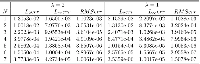
The linear system (3.2) is solved using the proposed scheme forλ= 1,2. We solve this problem with several values ofN andNe. Table1 shows the errors of proposed
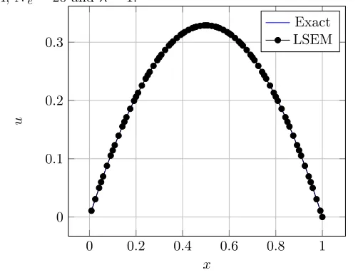
scheme with several values ofN andNe= 20. Figure1 show graph of exact solution
and approximate solution withN= 4 and Ne= 20.
Table 1. Numerical results for Bratu’s problem withNe= 20.
λ= 2 λ= 1
N L2err L∞err RM Serr L2err L∞err RM Serr
1 1.3053e-02 1.6500e-02 1.1023e-03 2.1529e-02 2.2097e-02 1.1028e-03 2 1.0018e-02 7.9776e-03 3.0531e-04 1.3130e-02 8.3774e-03 3.2024e-04 3 2.2023e-03 9.9553e-04 3.6104e-05 2.4071e-03 1.0268e-03 3.9460e-05 4 3.9778e-04 1.9421e-04 4.9109e-06 6.4771e-04 3.4862e-04 7.9964e-06 5 2.5862e-04 1.3858e-04 3.5507e-06 1.0154e-04 5.3085e-05 1.0053e-06 6 1.5050e-04 1.0004e-04 2.8967e-06 3.5765e-05 1.5567e-05 2.9558e-07 7 3.7733e-05 4.2734e-05 1.0061e-06 3.5359e-06 1.0017e-05 1.5078e-07
5. Conclusion
Figure 1. Exact and numerical results for Bratu’s problem with N = 4, Ne= 20 andλ= 1.
0 0.2 0.4 0.6 0.8 1 0
0.1 0.2 0.3
x
u
Exact LSEM
accuracy. In this article, we constructed a LSEM for the solution of the Bratu’s problem. We used the LSEM for discretizing the spatial space. Also we used a quasi-linearization method for linearised the problem. Finally, using the test problems, we demonstrated that the algorithm is efficient for obtaining approximation solutions of Bratu’s problem.
References
[1] S. Abbasbandy, M. S. Hashemi and C. S. Liu,The Lie-Group shooting method for solving the Bratu’s equation, Commun. Nonlinear Sci. Numer. Simul.,16, (2011), 4238–4249.
[2] S. O. Adesanya, S. A. Arekete and E. S. Babadipe,A new result on Adomian decomposition method for solving Bratus problem,Math. Theory Model,3(1), 92013), 116–120.
[3] Q. Ai, H. Y. Li and Z. Q. Wang,Diagonalized Legendre spectral methods using Sobolev orthog-onal polynomials for elliptic boundary value problems, Appl. Numer. Math., (2018).
[4] K. J. Bathe,Finite Element Procedures, second ed., Prentice-Hall, Englewood Cliffs, NJ, (1995). [5] R. E. Bellman and R. E. Kalaba,Quasilinearization and Nonlinear Boundaryvalue Problems,
Elsevier, New York, (1965).
[6] M. Ben Romdhane and H. Temimi, An iterative finite difference method for solving Bratu’s problem, J. Comput. Appl. Math.,292, (2016), 76–82.
[7] J. P. Boyd,An analytical and numerical study of the two-dimensional Bratu’s equation, J. Sci. Comput.,1(12), (1986), 183–206.
[8] G. Bratu,Sur les equation integrals non-lineaires, Bull. Math. Soc. France.,42, (1914), 113–142. [9] R. Buckmire, Investigations of nonstandard, Mickens-type, finite-difference schemes for sin-gular boundary value problems in cylindrical or spherical coordinate, Numer. Methods Partial Differential Equations,19, (2003), 380–398.
[10] Y. Chen, N. Yi and W. Liu,A Legendre–galerkin spectral method for optimal control problems-governed by elliptic equations, Siam J. Numer. Anal.,46, (2008), 2254–2275.
[12] R. Courant,Variational method for the solution of problems of equilibrium and vibration, Bull. Am. Math. Soc.,49, (1943), 1–23.
[13] M. A. El Tawil and H. N. Hassan,An efficient analytic approach for solving two point nonlinear boundary value problems by homotopy analysis method, Math. Methods Appl. Sci.,34, (2006), 977–989.
[14] F. X. Giraldo, Strong and weak Lagrange-Galerkin spectral element methods for the shallow water equations, Comput. Math. Appl,45, (2003), 97–121.
[15] Q. Guo, N. Pan and Y. Q. Wan,Thermo-electro-hydrodynamic model for electrospinning pro-cess, Int. J. Nonlinear Sci. Numer. Simul.,5, (2004), 5–8.
[16] A. Hamdan and M. I. Syam,An efficient method for solving Bratu’s equations, Appl. Math. Comput.,176, (2011), 704–713.
[17] J. S. Hesthaven, S. Gottlieb and D. Gottlieb,Spectral Method for Time-Dependent Problems, Cambridge University Press, (2007).
[18] J. Jacobsen and K. Schmitt,The Liouville-Bratu-Gelfand problem for radial operators, J. Dif-ferential Equations,174(1), (2002), 283–298.
[19] . A. Khan, C. S. Upadhyay and M. Gerritsma,Spectral element method for parabolic interface problems, Comput. Methods Appl. Mech. Engrg, (2018).
[20] S. Liao and T. Tan, A general approach to obtain series solutions of nonlinear differential equations, Stud. Appl. Math.,119, (2007), 297–354.
[21] M. Lotfi and A. Alipanah,Legendre spectral element method for solving sine-Gordon equation, Advances in Difference Equations,119, (2019). DOI 10.1186/s13662-019-2059-7.
[22] Y. Maday and A. T. Patera,Spectral Element Methods for the Incompressible Navier-Stokes Equations, Surveys on Computational Mechanics, ASME, New York (1989).
[23] A. Mohsen, A simple solution of the Bratu’s problem, Comput. Math. Appl, 67(1), (2014), 26–33.
[24] A. T. Patera,A spectral element method for fluid dynamics: laminar flow in a channel expan-sion, J. Comput. Phys.,54, (1984), 468–488.
[25] C. Pozrikidis,Introduction to Finite and Spectral Element Methods Using Matlab, Chapman and Hall/CRC, (2005).
[26] E. Priolo and G. A. Seriani,A numerical investigation of Chebyshev spectral element method for acoustic wave propagation, Proceedings of the 13th IMACS Conference Comparat., (1991), 154–172.
[27] S. Sandile, M. Motsa and S. Precious, Some modifications of the quasilinearization method with higher-order convergence for solving nonlinear BVPs, Numer. Algorithms,63(3), (2013), 399–417.
[28] A. Serghini Mounim and B. M. De Dormale,From the fitting techniques to accurate schemes for the Liouville-Bratu-Gelfand problem, Numer. Methods Partial Differential Equations,22(4), (2006, 761–775.
[29] F. N. Van de Vosse and P. D. Minev,Spectral Element Methods: Theory and Aplications, EUT Report 96-w-001, Eindhoven University of Technology, (1996).
[30] R. G. Vano and T. N. Phillips,The choice of spectral element basis functions in domains with an axis of symmetry, J. Comput. Appl. Math,201, (2007), 217–229.
[31] Y. Wang, G. Qin and Z. Q. Wang,An improved time-splitting method for simulating natural convection heat transfer in a square cavity by Legendre spectral element approximation, Com-puters and Fluids, (2018).
[32] C. Xu and Y. Maday,A spectral element method for the time-dependent two-dimensional Euler equations: applications to flow simulations, J. Comput. Appl. Math,91, (1998), 63–85. [33] E. Zampieri and L. F. Pavarino,Approximation of acoustic waves by explicit Newmark’s schemes
and spectral element methods, J. Comput. Appl. Math.,185, (2006), 308–2006.