Multiple Signal Detection using the ESPRIT Algorithm



Abstract—An array antenna system with innovative signal processing to estimate the direction of arrival (DOA) for multiple targets is investigated in this paper. The signal processing technique in this study is the ESPRIT (estimation signal parameter via a rotational invariant technique). The DOA angles are derived indirectly from the generalized eigenvalues of the auto-correlation and cross-correlation matrices. Two different methods to estimate the multi-signal’s DOA are: (1) Choice of a proper set of generalized eigenvalues from the two sub-arrays and (2) Choice of an appropriate proper set of generalized eigenvectors from the two sub-arrays. The estimated autocorrelation and cross correlation matrices in this study is based on combination of temporal averaging and spatial smoothing method. Extensive computer simulations are used to demonstrate the performance of the processing algorithms.

Index Terms—DOA estimation, array antenna, advanced signal processing.

I. INTRODUCTION

Accurately estimating the direction of arrival (DOA) has many important applications in communication and radar systems. Using the conventional fixed antenna, the resolution of DOA is limited by the antenna mainlobe beamwidth. Using the array antenna and advanced signal processing techniques, the DOA estimation variance can be greatly reduced.

Two important classes of signal processing techniques are the model based approach and the eigenanalysis method[1]. The model based method assumes that the received data is modeled as the output of a linear shift invariant system. The DOA information may be obtained indirectly from the estimated model parameters. Several eigen-analysis methods such as multiple signal classification (MUSIC)[2], polynomial root intersection for multidimensional estimation (PRIME)[3,4] have been investigated by several authors. This paper is a study of multi-signal’s DOA estimation using the ESPRIT[5,6,7] algorithm. DOA estimation of a single

Manuscript received March 10, 2010. This work was supported in part by the Raytheon Space and Airborne Systems.

Alfred Tsz Yin Lok is s graduate students at the Electrical and Computer Engineering Department, California State Polytechnic University, Pomona, CA 91768.

Z. Aliyazicioglu is with the Electrical and Computer Engineering Department, California State Polytechnic University, Pomona, CA 91768 USA, phone: 909-869-3667; fax: 909-869-4687; (e-mail: zaliyazici@ csupomona.edu).

H. K. Hwang is with the Electrical and Computer Engineering Department, California State Polytechnic University, Pomona, CA 91768 USA phone: 909-869-2539; fax: 909-869-4687; (e-mail: [email protected]).

target using ESPRIT method is fairly straightforward. A signal’s DOA can be derived from the maximum generalized eigenvalue[6] of two independent equations. If there are multiple targets, determining the signal DOA depends on the choice of an appropriate pair of generalized eigenvalues from two independent equations. If the appropriate pair of generalized eigenvalues is not chosen, it results in a false DOA. Rather than choosing appropriate pairs based on the generalized eigenvalues, improved results can be obtained by choosing the appropriate pair based on the generalized vectors. A performance comparison is presented in this paper.

The array antenna used in this simulation study consists of 19 elements in a honeycomb configuration. In this paper DOA performance is discussed as a function of signal to noise ratio (SNR), and as an effect of spatial smoothing[8].

II. ESPRIT ALGORITHM

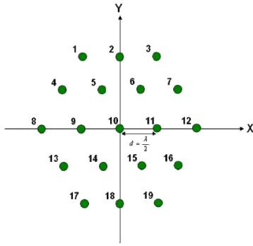
[image:1.612.334.513.455.629.2]

The array antenna considered in this paper has 19 antenna elements in a honeycomb configuration as shown in Figure 1. Array elements are uniformly placed on an x-y plane. The inter-element spacing d equals half of the signal wavelength.

Figure 1 Two Dimensional Arrays with 19 Elements Assume the nth _{narrowband signal is impinging on the array}

from an elevation angle n and azimuth angle n as shown in

Figure 2. Using the nth _{signal received by the center element}

snc(t) as the reference, the nth signal received by the ith element

sni(t) is

Multiple Signal Detection using the ESPRIT

Algorithm

[image:2.612.103.283.517.675.2]

Figure 2 Coordinate of array system and signal direction

sni(t) = snc(t)

e

jβni (1)

where the electrical angle of the ith _{element } ni is

) sinφ

y cosφ

sinθ(x

λ

2π

-

β_ni _{i n} _{i n} (2)

where (xi, yi) are the coordinates of the ith element.

Equation (2) shows that the signal DOA angles (n, n) are

related to the electrical angle ni. The ESPRIT algorithm

derives the DOA angles from the phase factor . Determining two angles (n, n) requires two different phase factors. Two

independent phase factors can be derived from two independent position shifts. A brief description of ESPRIT using a 19 element array is as follows:

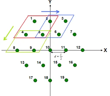
An appropriate subset is chosen from the original array and this subset is shifted in two different directions. The subset in this study consists of element (1, 2, 4, 5). The data vectors of the subset and shifted subsets (2, 3, 5, 6) and (4, 5, 8, 8) are related by the appropriate electrical angles. The signal’s elevation and azimuth angles can be derived from the two electrical angles corresponding to the two different shifts. The subset and two different shifts used in this study are shown in Figure 3.

Figure 3. Subset and Two Linearly Shifted Subsets Now , assume there are two independent narrowband signals impinging on the antenna from DOA (1, 1) and (2,

2), respectively. The waveform y received by the subset

consists of elements (1, 2, 4, 5) and can be expressed as:

y(n) = s1,10(n)s1 + s2,10(n)s2 + wy(n) (3)

where wy(n) is the random white noise and wy(n) = [w1(n),

w2(n), w4(n), w5(n)]T, s1,10(n) is the signal received by the

center element due to signal 1, s2,10(n) is the signal received

by center element due to signal 2, s1 =

[

e

jβ1,1_,

e

jβ1,2_,

e

jβ1,4_,

e

jβ1,5_]T_{, s}

2 = [

e

jβ2,1,

e

jβ2,2,

e

jβ2,4,

e

jβ2,5]T.

The correlation matrix Ryy of this subset is

Ryy = E[yyH] =







           H 2 H 1 2 1 2

1 _{0 P}

0 P

s s s

s + 2

w

σ I (4)

where P1 and P2 are the power of signal 1and 2, respectively

and 2 w

σ is the noise variance.

Shifting this subset horizontally to the right forms a new subset consisting of elements (2, 3, 5, 6). The received waveform of this new subset z(n) is

 (n)

z s1,10(n)s3 + s2,10(n)s4 + wz(n) (5)

where wz(n) = [w2(n), w3(n), w5(n), w6(n)]T is the noise vector, s3 = 1,11

jβ

e

s1, s4 = 2,11

jβ

e

s2.

The cross correlation matrix Ryz is

Ryz = E[yzH] =





_

           H 2 jβ -H 1 -jβ 2 1 2 1 2,11 1,11 e e P 0 0 P s s s

s + σ2wQ (6)

where Q =

            0 1 0 0 0 0 0 0 0 0 0 1 0 0 0 0

Arranging the eigenvalues of matrix Ryy 1, 2, 3, 4 in

descending order, the noise variance

σ

2_w can be estimated by the following equation.

2 w

σ

= (3 + 4)/2 (7)

Define matrices Cyy and Cyz as

Cyy = Ryy -

σ

2_wI =





_

           H 2 H 1 2 1 2 1 P 0 0 P s s s

s (8)

Cyz = Ryz -

σ

2_wQ =





_

           H 2 jβ -H 1 -jβ 2 1 2 1 _2,11 1,11 e e P 0 0 P s s s

s (9)

Then Cyy –Cyz =













            H 2 jβ -H 1 -jβ 2 1 2 1 _2,11 1,11 e -1 e -1 P 0 0 P s s s s 

 , thus  =

1,11

jβ

e

and

_e

jβ2,11_{are two of the roots of det(C}

yy – Cyz). Two

phase factors 1,11 and 2,11 can be obtained by finding the

n

two roots of det(Cyy – Cyz) closest to the unit circle.

Forming subset (4, 5, 8, 9), the second independent phase factor can be obtained. The received data vector of this subset

v is:

(n) e

e

(n) v

jβ

jβ1,14 _s  2,14 _s _w

 s_1,10(n) ₁ s_2,10(n) ₂

v (10)

where wv(n) = [w4(n), w5(n), w8(n), w9(n)]T is the noise

vector.

The cross correlation matrix Ryv is Ryv = E[yvH] =





_

           H 2 jβ -H 1 -jβ 2 1 2 1 _2,14 1,14 e e P 0 0 P s s s

s + σ2wQ1 (11)

where Q1 =

            0 0 1 0 0 0 0 1 0 0 0 0 0 0 0 0

Define matrices Cyy and Cyv as:

Cyy = Ryy -

σ

_w2 I =

σ

2_sssH (12)

Cyv = Ryv -

σ

2_wQ1 =

σ

2_s

e

jβ8ssH (13)

Then Cyy –Cyv =













            H 2 jβ -H 1 -jβ 2 1 2 1 _2,14 1,14 e -1 e -1 P 0 0 P s s s s 

 , thus  =

1,14

jβ

e

and

_e

jβ2,14_{are two of the roots of det(C}

yy – Cyv). Two

phase factors

_e

jβ1,14_and

_e

jβ2,14_{can be obtained by finding the}

two roots of det(Cyy – Cyv) closest to the unit circle.

From n,11 = sinncosn, (14)

n,14 =

-2

π

sinncosn

3

sinn       

The electrical angles n,11, n,14 fornare obtained

from the appropriate pair of roots closest to unit circle from det(Cyy – Cyz) and det(Cyy – Cyv). Once we determine the

electrical angles n,11, n,14, the signal DOA can be obtained

by solving (n, n) from Equations (14) and (15).

III. MATRICES ESTIMATION

Section 2 shows that the DOA angles are derived from the auto-correlation and cross-correlation matrices. DOA performance depends on the accurate estimation of matrices

Ryy, Ryz, Ryv. Elements of matrices are estimated from the

received data y(n) = s(n) + w(n) where s(n) and w(n) are the signal and white noise of the received data. Three matrix estimation methods, (1) temporal averaging, (2) spatial smoothing, (3) temporal averaging and spatial smoothing, are described in this section [8].

A. Temporal Averaging Method

This method estimates the matrix element rij by averaging

the products of data received by the ith _{and j}th _{elements over N}

snapshots according to the following equation:

rij =

y

(n)y

(n)

N

1

N 1 n * j i



 (16)

B. Spatial Smoothing Method

Since the number of elements in the array is larger than the size of the subset, instead of discarding the data from elements outside of the subset, those data can be used to improve the estimation of rij. Any pair of elements that has a

similar geometrical relationship has the same spatial correlation. For example, elements of the correlation matrix of the square array for subset (1, 2, 4, 5) are computed from the following equations:

r11(n) = r22(n) = r44(n) = r55(n) = y(n)y(n) 19 1 19 1 i * i i



 (17)

There are 14 pairs of elements having the same correlation as r12(n), thus r12(n) can be computed from the following

equation.





(n) (n)y y (n) (n)y y (n) (n)y y (n) (n)y y 14 1 * 19 18 * 5 4 * 3 2 * 2 1       (n)

r_{12 (18)}

Other elements of the correlation matrix can be computed in a similar manner.

C. Temporal Averaging and Spatial Smoothing Method

This method combines spatial smoothing and temporal averaging. After estimating the matrix elements rij(n) from

spatial smoothing, an estimated rij is obtained by further

averaging over N snapshots according to the following equation.

rij = r(n)

N 1 N 1 n ij



 (19)

IV. SIMULATION RESULTS

Assume that two tone signals are impinging on the array from (10o_{, 50}o_{) and (30}o_{, 120}o_{), where the first angle is the}

elevation angle and second angle is the azimuth angle. The signal to noise ratios of the first and second signals are 20 dB and 10 dB respectively. Since there are two signals, accurate DOA estimation relied on properly pairing the generalized eigenvalues of (Cyy, Cyz), and (Cyy, Cyv). Since the second

[image:4.612.76.304.48.191.2]

Figure 4. Histogram Based on Temporal Averaging over 32 Snapshots

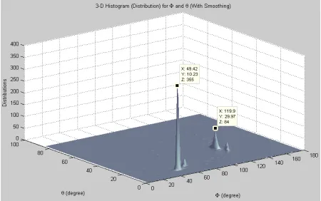
[image:4.612.319.540.50.193.2]

Figure 4 shows that the estimated DOA is quite noisy. This is due to the fact the estimated matrices are based on temporal averaging over 32 snapshots. Increasing the number of snapshots should improve the DOA estimation. However, when operating the system in real time the number of snapshots is usually limited. Improved DOA performance can be achieved by matrices estimation using a combination of temporal averaging and spatial smoothing. Figure 5 shows the estimated DOA histogram by matrices estimation using temporal averaging and spatial smoothing.

Figure 5. Histogram Based on Temporal Averaging over 32 Snapshots and Spatial Smoothing

Figure 5 shows that the two clear peaks are very close to the signal DOA. The stronger peak is close to the stronger signal DOA at (10o_{, 50}o_{). Figures 4 and 5 show that enhanced}

matrices estimation by combination of temporal averaging and spatial smoothing improves the performance of ESPRIT algorithm.

If the two signals have the same power, estimating the signal’s DOA using an inappropriate pair of eigenvalues may create a false DOA. Figure 6 shows the histogram of two signals with the identical SNR = 20 dB.

Figure 6. Histogram Based on Temporal Averaging over 32 Snapshots and Spatial Smoothing

Since the two signals have the same amount of power, the probability of estimating signal DOA using an incorrect pair of generalized eigenvalues is fairly high. Thus Figure 6 shows that there are two false peaks due to having chosen the wrong pair of generalized eigenvalues.

Rather than define the correct pair of eigenvalues based on their relative distance from the unit circle, we can use the generalized eigenvectors to define the appropriate pair. Suppose the generalized eigenvalues of (Cyy, Cyz) are 1, 2

and their associated eigenvectors are q1 and q2, the

generalized eigenvalues of (Cyy, Cyv) are a, b and their

associated eigenvectors are qa and qb. If the Euclidean

distance between q1 and qa is less than the Euclidean distance

between q1 and qb, then we pair (1,a) and (2,b) to

compute the signal DOA. Otherwise we pair (1,b) and

(2,a) to compute the signal DOA. Based on this method,

[image:4.612.76.301.362.503.2]

the estimated DOA histogram is shown in Figure 7.

Figure 7. Histogram Based on Temporal Averaging over 32 Snapshots and Spatial Smoothing

[image:4.612.318.542.447.576.2]

V. CONCLUSION

The conclusions based on the results of this simulation study are summarized as follows:

1.The ESPRIT method estimates signal DOA by finding the roots of two independent equations closest to the unit circle. This method does not require using a scan vector to scan over all possible directions like the MUSIC (Multiple Signal Classification) algorithm.

2.Performance of DOA estimation can be enhanced by improved matrices estimation. One method to improve matrices estimation is to estimate matrices by combination of temporal averaging and spatial smoothing.

3.When there is a large difference between the powers of two signals, choosing the first pair of eigenvalues as the one closest to unit circle and the second pair of eigenvalues as the second closest to unit circle provides a reasonable DOA estimation.

4.When the powers of two signals are identical, pairing the eigenvalues based only on their distance to the unit circle may create false peaks. An improved DOA estimation can be obtained by choosing the pair of eigenvalues whose associated eigenvectors have minimum Euclidean distance.

5.Array element position may deviate from the ideal position. Position deviation will degrade DOA performance. Sensitivity analysis due to imprecise element position will be carried out in a future study.

ACKNOWLEDGMENT

The authors would like to thank the Raytheon Space and Airborne Systems for its support of this investigation.

REFERENCES

[1] J. Proakis, D. K. Manolakis Digital Signal Processing, Prentice Hall, 2006, 4th Ed

[2] R.O Schmidt, "Multiple Emitter Location and Signal Parameter Estimation," IEEE Trans. Antennas Propagation, Vol. AP-34 [3] M. Pesivento, A. B. Gershman, M. Haardt, “A Theoretical and

Experimental Study of a Root MUSIC Algorithm based on a Real Valued Eigen decomposition”

[4] Z. Aliyazicioglu, H. K. Hwang, M. Grice, A. Yakovlev, ”Sensitivity Analysis for Direction of Arrival Estimation using a Root-MUSIC Algorithm” Engineering Letters, 16:3, EL_16_3_13

[5] G. F. Hatke, K. W. Forsythe, “A class of polynomial rooting algorithms for joint azimuth/elevation estimation using

multidimensional arrays” Signals, Systems and Computers, 1994. 1994 Conference Record of the Twenty-Eighth Asilomar Conference [6] Z. Aliyazicioglu, H. K. Hwang, “Performance Analysis for DOA

Estimation using the PRIME Algorithm” 10th International Conference on Signal and Image Processing, 2008

[7] R. Roy, T. Kailath, “ESPRIT-estimation of signal parameters via rotational invariance techniques” IEEE Transactions on Acoustics, Speech and Signal Processing, 1989