DESERT Online at http://jdesert.ut.ac.ir
DESERT 19-1 (2014) 1-9
Evaluation of Different Cokriging Methods for Rainfall
Estimation in Arid Regions (Central Kavir Basin in Iran)
M.A. Zare Chahouki
a, A. Zare Chahouki
b*, A. Malekian
a, R. Bagheri
c, S.A. Vesali
ca
Department of Rehabilitation of Arid and Mountainous Regions, University of Tehran, Karaj, Iran
b Faculty of Natural Resource Management, Yazd University, Yazd, Iran c
MENARID provincial project manager of Yazd Province, Yazd, Iran
Received: 6 February 2010; Received in revised form: 7 January 2014; Accepted: 15 January 2014
Abstract
Rainfall is cons idered a highly valuable climatologic resource, particularly in arid regions. As one of the primary inputs that drive watershed dynamics, rainfall has been shown to be cru cial for accurate distributed hydrologic modeling. Precipitation is known only at certain locations; interpolation procedures are needed to predict this variable in other regions. In this study, the ordinary cokriging (OCK) and collocated cokriging (CCK) m ethods of interpolation were applied for rainfall depths as the primary variate associated with elevation and surface elevation values as the s econdary variate. The different techniques were applied to monthly and annual precipitation data
measured at 37 meteorological stations in the Central Kavir basin. These sequential stepswere repeated for the mean
monthly rainfall of all twelve months and annual data to generate rainfall prediction maps over the study region. After carrying out cross-validation, the smallest prediction errors were obtained for t he two mult ivariate geostatistical algorithms. The cross-validation error statistics of OCK and CCK p resented in term s of root m ean square error (RMSE) and average error (AE) were within the acceptable limits for most months. Then the two approaches were compared to select of the most accurate method (AE close to zero and RMSE from 0.53 to 1.46 for 37 rain gauge locations for all months). The exploratory data analysis, variogram model fitting, and generation precipitation prediction map were accomplished through use of ArcGIS software.
Keywords: Altitude; Central Kavir basin; Cokriging; geographical information system; Precipitation
1. Introduction
Most of the water received by a river basin occurs as rainfall events over the basin. As one of the primary inputs that drive watershed dynamics, the estimation of spatial variability of precipitation has been shown to be crucial for accurate distributed hydrologic modeling. The estimation of precipitation, accordingly, is very important for assessing water resources. The estimation of precipitation is also important for predicting natural hazards caused by heavy rain. To estimate precipitation properly, it is necessary to have o ptimally distributed rain gauges and to apply an a ppropriate technique
Corresponding author. Tel.: +98 351 8123245, Fax: +98 351 8123245.
E-mail address: [email protected]
precipitation estimation in a 52 000 km2 region
in Nebraska and Kansas.
According to Ahmed and De Marsily (1987), kriging with external drift (KED) is more adapted than ordinary kriging for coarse sampling data. It lies in the adoption of an external variable which is observed with a spatial density exceeding that of t he original variable. Grimes et al. (1999) adopted kriging
with external drift using both satellite data and ground rain gauges to improve the estimation of decadal rainfall and their spatial distribution while Goovaerts (2000) adopted a digital elevation model for monthly and annual rainfall totals in south Portugal.
Hevesi et al. (1992a, b) analyzed annual
precipitation estimates with geostatistical techniques. Then they used cokriging to estimate the precipitation distribution as a function of elevation. Compared with other techniques, they found that cokriging gave the best estimate. Creutin et al. (1988) introduced a
simplified cokriging system to optimize merging radar rainfall and rain gauge data and found it very effective in reducing system size. Phillips et al. (1992) compared three
geostatistical procedures for spa tial analysis of precipitation in m ountainous terrain in western Oregon (Willamette River basin). Detrended kriging and cokriging compared with kriging offer improved spatially distributed precipitation estimates in mountainous terrain on the scale of a few million hectares.
PardoIgu´zquiza (1998) compared the areal average climatological rainfall mean estimated by the classical Thiessen method, ordinary kriging, cokriging, and kriging with an external drift (the first two methods used only rainfall information, while the latter two used both precipitation data and orographic information) in the G uadalhorce river basin in so uthern Spain, and concluded that kriging with an external drift seemed to give the most coherent results in accordance with cross-validation statistics and had the advantage of requiring a less demanding variogram analysis than cokriging.
Goovaerts (2000) compared TP, WMA, ordinary kriging with varying local means, kriging with external drift and collocated co-kriging for spatial interpolation of monthly and annual rainfalls. The r esults showed large prediction errors of the TP and WMA, while ordinary kriging was more accurate.
Diodato and Ceccarelli (2005) compared the inverse squared distance method with linear regression and ordinary cokriging (OCK) for the Sannio Mountains (southern Italy), obtaining
the best results with cokriging that included elevation as secondary information.
Diodato (2005) studied the influence of topographic co-variables on t he spatial variability of precipitation over small regions of complex terrain. The results showed that ordinary cokriging is a very flexible and robust interpolation method, because it may take into account several properties (soft and hard data) of the landscape.
Li et al., (2006) estimated daily suspended
sediment loads (S) using cokriging (CK) of S with daily river discharge based on weekly, biweekly, or monthly sampled sediment data. The results showed that the estimated daily sediment loads with CK using the weekly measured data best matched the measured daily values.
Hengl et al. (2007) discussed the
characteristics of re gression-kriging (RK) or Universal Kriging, its strengths and limitations, and illustrated these with a simple example and three case studies.
Portal´es et al. (2009) performed a
comparative study of different univariate and multivariate interpolation in e astern Spanish Mediterranean coast. Models were achieved for seasonal scales, considering a total of 179 rain gauges; data from another 45 rain gauges were also used to predict errors. Results proved that there is no ideal method for all cases; the method to be used will depend on (a) the number of geographical factors that influence rainfall, and (b) the m ajor or minor s patial correlation within the rainfall.
Zhang and Srinivasan (2009) developed nearest-neighbor (NN), inverse distance weighted (IDW), simple kriging (SK), ordinary kriging (OK), simple kriging with local means (SKlm), and k riging with external drift (KED) to facilitate the estimation of automatic spatial precipitation while incorporating the geographic information system program in the Luohe watershed, located downstream of the Yellow River basin. The evaluation results showed that the SKlm_EL_X and KED_EL_X methods, which incorporate elevation and spatial coordinates into SKlm and K ED, respectively, produced significantly better results than Thiessen polygon and IDW in ter ms of th e coefficient of correlation.
secondary variate, 2. to a ttempt different CK methods and se lect the best one through analyzing the cross-validation error statistics through cross-semivariogram models, and 3. to use the selected CK method to predict rainfall values at unmeasured locations.
The benefits of a geographical information system (GIS) and a geostatistics approach to accurately model the spatial distribution pattern of precipitation are known.
2. Materials and Methods
The study area is located in the center of Iran (latitude between 34º 15´and 36º 56´N, longitude between 52º 15´and 56º 53´ E) on the southern border of the Alborz mountain range. Central Kavir basin is one of the largest regions in Iran’s central zone. The study area is part of this basin with a surface area of approximately 57784 km2. To the north lie districts within the
Alborz mountain range. The maximum and minimum altitudes in the region are 3884 and 648 m a.s.l., respectively. The mean altitude is about 1238 m a .s.l. Figure 1 sh ows the DEM, with a spatial resolution of 50 m, used in this research.
Mean annual precipitation reaches approximately 180 mm i n the majority of the areas of the region, ranging from <70 mm in the
south of the study region to as much as >300
mm in the northern mountainous areas. One of the most important characteristics of the
precipitation is it s interannual variability. The region has a dry season from June to November and a wet season from December to May (>80% of the precipitation falls between these months). Kavir basin is an arid region where the water balance is negative.
The delineated base map (i.e. polygon feature class) of the study area and the location of rainfall gauging stations within the Kavir basin (i.e. point feature class) were generated using ArcGIS as two different coverage feature classes. The point feature class coverage map, representing the rainfall locations, also contained the mean monthly rainfall depths for twelve months as attribute values. The base map and the rainfall point coverage map were overlaid to represent the rain gauge locations. The DEM of study area was use d to extract approximately 160 elevation points ranging from of 670 to 3600 m a.s.l. covering the entire study area for use i n co-kriging analysis. The geostatistical analysis extension module of ArcGIS 9.3 was used to analyze and develop kriged surfaces. Several interpolation approaches are available in geographical information systems (GISs) to meet the general requirements of i nterpolation. Figure 1 shows the spatial distribution of the rain gauge stations and the locations of 160 extracted elevation points from DEM with elevations used in this study. Many stations are situated in mountainous areas.
Daily precipitation data for 30 years (1971-2004) were obtained from 37 meteorological stations. Rainfall measurements are collected daily and compiled to generate monthly totals. Estimating rainfall depth at unsampled locations can be i mproved by interpolating between the nearest gauges. The daily observations made at all stations pass through a rigoro us quality control procedure. Consistency checks were applied to the data. After assuring the quality of
the raw data, monthly precipitation averages were calculated. Some basic sample statistics were also determined (Table 1). Data used in the analysis were derived from Iran’s Ministry of Energy. The analysis of the primary variate (mean monthly rainfall depth) and secondary variate (elevation) resulted in good correlation values, ranging from 0.50 (January) to 0.77 (September).
Table 1. Descriptive statistics of the monthly and annual precipitation (mm) data for 37 meteorological stations month Mean Median deviation Standard Maximum value Minimum value of skewness Coefficient Kurtosis Co*
January 20.26 19.10 7.63 41.90 8.20 0.86 0.69 0.50
February 22.81 20.20 8.75 39.90 9.40 0.52 -0.80 0.73
March 28.97 28.60 1.60 50.40 9.10 0.30 -0.16 0.70
April 27.10 25.30 9.57 48.20 9.70 0.51 -0.61 0.69
May 22.49 18.70 11.04 44.70 5.90 0.53 -0.87 0.75
June 7.37 5.10 5.76 24.40 0.20 1.21 0.89 0.73
July 4.84 3.80 4.16 15.40 0.30 1.11 0.46 0.74
August 3.54 2.20 3.25 11.80 0.10 1.24 0.59 0.75
September 3.57 2.60 2.93 10.80 0.00 0.85 -0.17 0.77
October 6.99 5.40 4.98 18.90 1.50 0.99 -0.36 0.69
November 12.35 9.50 8.09 33.30 3.10 1.35 0.81 0.62
December 20.94 18.40 9.73 57.00 7.50 1.61 3.95 0.72
Annual 181.41 154.92 76.24 348.54 73.54 0.80 -0.43 0.78
*: Cor = Linear correlation coefficient between precipitation and altitude.
2.1. Geostatistical interpolation techniques
In this section, the estimators used i n the case study are briefly introduced. More information about them can be found in Goovaerts (1997). All geostatistical estimators are variants of the linear regression estimator Z*(x):
( ) ( )
). ( )
( ) (
1 *
i i n
i
i x Z x m x
w x m x
Z
(1)
where each datum, Z(xi ), has an associated
weight, wi(x), and m(x) and m(xi ) are the
expected values of Z*(x) and Z(xi ), respectively.
The kriging weights must be determined to minimize the estimation variance, Var [Z*(x) -Z*(x)], while ensuring the unbiasedness of the
estimator, E[Z*(x)- Z*(x)] = 0. All different types
of kriging are distinguished depending on the chosen model for the trend, m(x), of the random
function Z(x) (Goovaerts, 1997).
In this study, three phases were completed to conduct any geostatistical work (Moral, 2009):
1. Exploratory analysis of data. Data were
studied without considering their geographical distribution. Statistics were applied to check data consistency, remove outliers, and identify the statistical distribution from where the data came.
2. Structural analysis of data. Spatial
distribution of the variable was analyzed.
Spatial correlation or dependence can be quantified with semivariograms.
A variogram shows the degradation of spatial correlation between two points of space when the separation distance increases. Function has two components: i) the nugget effect, which characterizes the discontinuity jump observed at the origin of distances and quantifies the short-term, erratic variations of the studied phenomenon plus measurements and data errors; ii) the increasing part of the variogram, which may reach the sill (theoretical sample variance), level off the curve, for a distance called range, or incr ease continuously with distance. The non-nugget part of the variogram measures the non-random part of the phenomenon and models its average medium-scale behavior in space.
The variogram is a function of both distance and direction, and so direction-dependent variability can be accounted for.
possible way to incorporate secondary data. Although it is indicated when the secondary information is not exhaustive, i.e. auxiliary data are not available at all grid-nodes, if this information is known everywhere and c hanges smoothly across the study area, the cokriging system can retain only the secondary datum collocated with the location which is estimated (Goovaerts, 1997). In the current study we performed two cokriging methods. Ordinary co-kriging is the estimation of one variable based on the measured values of two or more variables. It is a ge neralization of kriging in the sense that at every location there is a vector of many variables instead of one variable. OCK is the multivariate extension of kriging (Goovaerts, 1997). OCK analysis was performed for the 37 primary data points and the secondary variate (elevation points extracted from the DEM). Collocated ordinary co-kriging is a conditional estimator of CK where the neighborhood uses the secondary variable as a subset of l ocations where primary data are available along with the estimated locations (Wackernagel, 2003). The primary variate of the 37 measured values of precipitation and the corresponding altitude values were used in the analysis. CCK analysis was performed for 41 primary data points (precipitation) and the secondary variate was the elevation of the point locations included in th e primary variate [See Goovaerts (1997) for a detailed presentation of cokriging algorithms].
All geostatistical analyses were conducted using the extension Geostatistical Analyst of the GIS software ArcGISd (version 9.3, ESRI Inc). After modeling annual and m onthly precipitation with the selected algorithms, a set of map layers in raster format was generated.
2.2. Error statistics
The performances of th e OCK and CCK algorithms were assessed and compared using cross-validation results. This was achieved by temporarily removing one datum at a time from the data set and re-estimating the deleted value from the remaining data using kriging algorithms. In the present study, the reduced mean square error (RMSE) a nd the average error (AE) were the error statistics used (Campling et al., 2001) to compare the
model-predicted results with the observed values. RMSE was used to check the consistency between the estimation errors and the standard deviation of the observed values:
121 2 1
n i i i s p Z o Z nRMSE (2)
AE was used to test the predictability of the developed models:
n i i i s p Z o Z n AE 11 (3)
where:
zoi = observed value at location i zpi = predicted value at i
N = number of pairs of observed and predicted values
S = standard deviation of the observed values. This RMSE value should be within the range of 1 ±[2(2/N)1/2] for the model to be acceptable
(Ella et al., 2001). The AE value should be
close to zero for the model to be acceptable.
3. Results
The exploratory data analysis performed on the primary variate and the secondary variate of elevation revealed that the da ta are normally distributed and free of outliers. In cokriging, the primary and secondary variates were fitted using different models available in the ArcGIS geostatistical extension module, and the optimal cross-semivariogram was selected. Figures 2 and 3 show annual and monthly semivariograms.
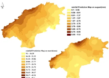
After calculating OCK and CCK, the cross-validation error statistics were compared to select the best method to perform the CK, Then, the best CK algorithm (either OCK or CCK) was used to predict the primary variate values for more locations within the study region. The database of these predicted variables corresponding to ele vation locations provided the rainfall depths at predicted unmeasured locations. The cross-validation statistics in terms of R MSE and AE were estimated to ascertain the model algorithms, and finally the interpolated surface reflecting the variation of rainfall depth over the study area was generated using ArcGIS. These procedures were followed to generate the spatial variability map of long-term mean monthly rainfall for one m onth and replicated for all twelve months to ge nerate twelve such maps. The interpolated surface was generated for the study region for the twelve months, and the map of annual rainfall, driest (august) and wettest (March) months of the year are presented in Figures 4 and 5, respectively.
Fig. 2. Annual Rainfall Semivariogram
Fig. 3. Monthly Rainfall Semivariogram
0 804 1607 2411 3215
0.00 50809.31 101618.63 152427.94 203237.25
Se m iv a r ia nc e Separation Distance April 0 1080 2161 3241 4322
0.00 50809.31 101618.63 152427.94 203237.25
S e m ivar ia n ce Separation Distance May 0 581 1163 1744 2326
0.00 50809.31 101618.63 152427.94 203237.25
Se m iv a r ia nc e Separation Distance June 0 875 1750 2625 3500
0.00 50809.31 101618.63 152427.94 203237.25
S e mi var ia n ce Separation Distance March 0 787 1574 2361 3148
0.00 50809.31 101618.63 152427.94 203237.25
S e mi var ia n ce Separation Distance February 0 490 980 1470 1961
0.00 50809.31 101618.63 152427.94 203237.25
S e mi var ia n ce Separation Distance January 0 495 989 1484 1978
0.00 50809.31 101618.63 152427.94 203237.25
Se m iv a r ia nc e Separation Distance July 0 342 685 027 370
0.00 50809.31 101618.63 152427.94 203237.25 Separation Distance August 0 355 709 1064 1418
0.00 50809.31 101618.63 152427.94 203237.25
Se m iv a r ia nc e Separation Distance September 0 460 920 1380 1840
0.00 50809.31 101618.63 152427.94 203237.25
S e mi var ia n ce Separation Distance October 0 664 1328 1992 2656
0.00 50809.31 101618.63 152427.94 203237.25
S e mi var ia n ce Separation Distance November 0 912 823 735 646
0.00 50809.31 101618.63 152427.94 203237.25 Separation Distance December 0 7008 14016 21025 28033
0.00 50809.31 101618.63 152427.94 203237.25
This was performed to select the best method for predicting rainfall at unmeasured locations and to predict spatial variability. The cross-validation error statistics were estimated using Equations 2 and 3 to select the best model. The calculated RMSE of cross-validation results for a ll months were well within the acceptable range for the model obtained through the OCK and CCK method. Moreover, the AE
values calculated from the cross-validation results of the CCK and OCK algorithm methods for all months were close to zero. The cross-validation statistics performed for both the OCK and CCK methods of CK (Table 2) revealed that the OCK method performed better than the CCK method. Hence, the OCK algorithm was used to predict the rainfall prediction map.
Table 2. Comparison of OCK and CCK methods in terms of model fitting cross-validation statistics month Variogram model Cross-validation statistics ordinary cokriging collocated ordinary cokriging Cross-validation statistics
AEa RMSEb AEa RMSEb
January Exponential 0.032 1.02 0.036 1.03
February Exponential 0.016 0.73 0.009 0.82
March Exponential 0.013 0.76 0.040 0.95
April Exponential 0.005 0.93 0.014 0.98
May Exponential -0.016 0.74 0.005 0.90
June Exponential 0.004 0.81 0.018 0.89
July Spherical -0.003 0.74 -0.002 0.78
August Spherical 0.016 0.77 0.018 0.81
September Spherical -0.006 0.73 0.005 0.81
October Exponential 0.005 0.87 0.009 0.91
November Exponential 0.026 0.91 0.026 0.92
December Exponential 0.008 0.77 0.005 0.80
Annual Exponential 0.006 0.93 0.013 0.86
[a] The acceptable value of KAE is close to zero.
[b] The acceptable value of KRMSE (1 ±[2(2/N)1/2] is 0.53 to 1.46 (N = 37).
Fig. 5. Rainfall prediction map for the driest (August) and wettest (March) months
4. Discussion and Conclusion
Many studies, particularly those performed in Iran such as Zabihi et al., (2011), Mirmousavi et
al., (2010), Shaabani (2010), Saghafian et al.,
(2011), and Mahdavi et al., (2004) solely
compared IDW interpolation and kriging family approaches, and all of t he above-mentioned studies concluded that the kriging approach is best.
The mentioned researchers attempted to compare a deterministic method (IDW) with the univariate kriging family and concluded that the ordinary kriging method was the most appropriate technique. Some noted researchers the declared co-kriging to be the best among IDW and u nivariate kriging family techniques. The results of these comparisons are obvious. In many studies, concluded that the kriging method is most suitable, without regard to the origin of data and the point distribution. Comparison of interpolation approach while is worthwhile that the different methods from one family were compared.
In the current research, different geostatistical approaches were classified into deterministic, univariate kriging, and multivariate kriging categories. Then each method was compared within each family. For example, ordinary co-kriging (OCK) and collocated co-kriging (CCK) were compared
with each other and not compared with the deterministic approach.
It is understood that modeling rainfall spatial variability of an arid region with a s parse rain gauge network poses a challenging task in terms of prediction accuracy. Furthermore, the s hort observation record of so me stations and inconsistency in data recording also influence the rainfall predictability over the arid region. This necessitates the use of exploratory data analysis techniques as a pre requisite before using the data for geostatistical modeling. It also revealed the necessity of using some secondary variables such as altitude, proximity to large bodies of water, and land cover and the support of remote sensing.
Different multivariate kriging approaches used in this study to predict the spatial rainfall variability for arid regions with orographic effects are simple and reasonable approaches which can be applied to similar locations having sparse rain gauge locations and undulating topography.
the OCK and CCK methods were compared based on cross-validation error statistics.
The developed methodology of geostatistical analysis and mathematical association of rainfall and elevation values to estimate a standardized value for use in the CK method and the combination of OCK and CCK approaches to generate rainfall prediction maps can be applied to account for the spatial variability of rainfall.
References
Ahmed, S., G . De M arsily, 1987. Comparison of geostatistical methods for estimating transmissivity using data on transmissivity and specific capacity. Water Resources Research 23 (9), 1717–1737. Campling, P., A. Gobin, J. Feyen, 20 01. Temporal and spatial rainfall analysis across a humid tropical catchment. Hydrological Processes 15(3): 359-375. Creutin, J.D., C. Obled, 1982. Objective analyses and mapping techniques for rainfall field: an o bjective comparison. Water Resour. Res. 18; 413–431. Diodato, N., M. Ceccarelli, 2005. Interpolation processes using multivariate geostatistics for mapping of climatological precipitation mean in the Sannio Mountains (southern Italy). Earth Surface Processes and Landforms 30(3): 259–268, DOI:10.1002/ esp.1126
Diodato, N., 2005. The influence of topographic co- variables on the spatial variability of precipitation over small regions of complex terrain. International Journal of Climatology 25(3): 351–363, DOI: 10.1002/joc.1131
Ella, V.B., S.W. Melvin, R.S. Kanwar, 2001. Spatial analysis of NO3-N concentration in glacial till. Trans. ASA.
Goovaerts, P., 1997. Geostatistics for Natural Resources Evaluation. Oxford University Press: New York. Goovaerts, P., 2000. Geostatistical approaches for incorporating elevation into the spatial interpolation of rainfall. Journal of Hydrology 228; 113–129. Grimes, D.I.F., E. Pardo-Iguzquiza, R. Bonifacio, 1999.
Optimal areal rai nfall estimation using raingauges and satellite data. Journal of hydrology 222, 93–108. Hengl, T., Gerard B.M. Heuvelinkb, David G. Rossiter, 2007. About regression-kriging: From equations to case studies. Computers & Geosciences 33 (2007) 1301–1315.
Hevesi, J.A., A.L. Flint, J.D. Istok, 1992a.b. Precipitation estimation in mountainous terrain using multivariate geostatistics. Part I: structural analysis. J. Appl. Meteor. 31; 661-676.
Li Z., You-Kuan Zhang, Keith Schilling, Mary Skopec, 2006. Cokriging estimation of daily suspended sediment loads. Journal of Hydrology 327; 389-398.
Moral, F.J., 2009. Comparison of different geostatistical approaches to map cli mate variables: application to precipitation. Int. J. Climatol, 2009. DOI: 10.1002/joc.1913
Pardo-Ig´uzquiza, E., 1998. Comparison of geostatistical methods for estim ating the areal average climatological rainfall mean using data on precipitation and topography. International Journal of Climatology 18; 1031-1047.
Phillips, D.L., J. Dolph, D. Marks, 1992. A comparison of geostatistical procedures for spatial analysis of precipitation in mountainous terrain. Agric. For. Meteorol., 58:119-141.
Portal´es Cristina, Nuria Boronat,a Josep, E. Pardo- Pascuala, Angel Balaguer-Beserb, 2009. Seasonal precipitation interpolation at the Valencia region with multivariate methods using geographic and
topographic information. INTERNATIONAL
JOURNAL OF CLIMATOLOGY. DOI: 10.1002/joc Tabios, G.Q., J.D. Salas, 1985. A comparative analysis of techniques for spatial interpolation of precipitation. Water Resour. Bull. 21; 365–380.
Wackernagel, H., 2003. Mul tivariate geostatistics. In
Multivariate Geostatistics: An Intro duction with
Applications, 145-169. 3rded. New York, N.Y.: Springer-Verlag.