Modeling and solving a three-stage fixed charge transportation problem considering stochastic demand and price

(1)

Journal Vol. 2, N

www.jie

Mode

probl

N. Shira Abstrac This pap price. Th are prese destinati shortage demand. criteria s coefficie Keywor solution; Received: Revised: J Accepted:

1. Int

A su retailers compan in suppl (Diaby, of Industria No. 1, pp. 27

ems.icms.ac.

eling an

lem cons

azi 1, M. Sey

ct

per considers he objective ented here: v ion. Fixed ch e cost that inc . The model

scenario bas ent of variatio

rds

:

Fixed c ; mean; stand

: March 2014-1

July 2014-19

: August

2014-troductio

upply chain s and custo nies to custo

ly chain. Th 1991; Eski al Engineeri 7-40 .ir

nd solvin

sidering

yyed-Esfah

s a three-stag of the proble variable costs harge exists curs when th is formulate sed solution

on are comp

charge trans dard deviatio

12

-20

on

n is a netwo omers (N omers throu he cost of di

igun et al.,

ing and Ma

ng a th

stochast

hani 2 , H. So

ge fixed cha em is to max s that are rel

whenever th he manufactu ed as a mixed

approach to ared as the a

portation pro on; coefficien

ork of supp Jawahar & gh the ware istribution a 2005). The

nagement S

hree-stag

tic dema

oleimani 3,*

arge transpor ximize the pr ated to amou here is a tran urer does not d integer pro o find the o acceptable cr

oblem; stoch nt of variatio

pliers, manu & Balaji, 20 ehouses and

accounts for refore distr

Studies

ge fixed

and and p

rtation proble rofit for supp unt of transp nsfer from a

t have enoug ogramming p optimal solut riteria to deci

hastic optimi on.

ufacturers, 009). The d distributio

r about 30 p ribution pro

charge

price

em regarding plying deman portation cost

source to a gh products f problem and tion. Mean, ide about the

ization; mult

transporters problem o on centres is percent of th

blem is an

transp

g stochastic nds. Three ki

t between a s destination, for supplying d is solved us standard de e best solutio

ti-criteria sce

s, distributi of transport s an importa he product’ important p

ortation

(2)

N. Shirazi, M. Seyyed-Esfahani, H. Soleimani

Journal of Industrial Engineering and Management Studies (JIEMS), Vol. 2, No. 1 Page 28

transport homogeneous products from several sources to several destinations so that the total cost can be minimized . In a transportation problem, when fixed cost is also taken into account, the problem is known as fixed charge transportation problem (FCTP). The objective of an FCTP is to find the combination of routes that minimises the total distribution costs satisfying the supply and demand constraints (Vinay & Sridharan, 2012). So, the fixed-charge transportation problem is an extension of the classical transportation problem that considers two kinds of cost (variable and fixed costs) (Raj & Rajendran, 2011; Schaffer & O'Leary, 1989).Variable cost depends on per unit of transported and linearly increases with it. Fixed charge incurs whenever a nonzero quantity is transported from a source to a destination (Adlakha & Kowalski, 1999; N Jawahar & Balaji, 2009).In FCTP, the parameters (for example variable costs, fixed charges, price and demand) can be deterministic and Non-deterministic. Some research can be refer as deterministic (Adlakha, Kowalski, & Lev, 2010; N Jawahar & Balaji, 2009; N. Jawahar & Balaji, 2012; Lotfi & Tavakkoli-Moghaddam, 2013), etc. On the other hand, few works are undertaken with non-deterministic parameters in FCTP. Non-non-deterministic parameters can be different approaches such as fuzzy (Kundu, Kar, & Maiti, 2014; Yang & Liu, 2007), interval (Safi & Razmjoo, 2013), chaos, stochastic etc. To the best of our knowledge, there are not any works about FCTP when parameters of demand and price are stochastic in a 3-stage supply chain. In this paper, we focus on a 3-stage FCTP. We try to find quantity of transported products from a manufacturer plant to a distribution centre and from a distribution centre to a retailer and a retailer to a customer when the parameters of demand and price are nondeterministic to obtain maximum income.

The organization of this paper is as follows: Section 2 presents the literature review of FCTP to find gaps. Section 3 describes the mathematical model and its descriptions. Section 4 explains the solution methodology. Sensitivity analysis is presented in Section 5. Finally, in Section 6, conclusions are provided and some areas of further research are then stated.

2. Literature review

Literature review includes two sections: deterministic parameters and nondeterministic parameters in FCTP. Further, number of stages is considered in these two sections. There are many studies regarding deterministic parameters for FCTP. Review is categorised based on number of stage.

(3)

2011) formulate single stage fixed-charge problems with polynomials. Using polynomial formulations. They show structural similarity between different kinds of linear and fixed charge formulations. Lotfi and Tavakkoli-Moghaddam (Lotfi & Tavakkoli-Moghaddam, 2013) propose a genetic algorithm using priority-based encoding (pb-GA) for linear and nonlinear fixed charge transportation problems in which new operators for more exploration are proposed. They modify a priority-based decoding procedure proposed by Gen et al. (Gen, Kumar, & Ryul Kim, 2005)to adapt with the FCTP structure. Pintea et al. (Pintea, Sitar, Hajdu-Macelaru, & Petrica, 2012) describe some hybrid techniques for solving the fixed charged transportation problem. The problem is a two chain supply network. Classical nearest neighbor algorithm is used basically to find the best distribution centres.

Now we point some studies about FCTP with Non-deterministic parameters. A few works are done about uncertain FCTP. Safi and Razmjoo (Safi & Razmjoo, 2013) consider the fixed charge transportation problem under uncertainty, particularly when parameters are given in interval forms. All of parameters (i.e., variable costs, fixed charges, supply and demand parameters) are in interval forms. In this case it is assumed that both cost and constraint parameters are arrived in interval numbers. Considering two different order relations for interval numbers, two solution procedures are developed in order to obtain an optimal solution for interval fixed charge transportation problem (IFCTP). Kundu et al (Kundu et al., 2014) consider two fixed charge transportation problems with type-2 fuzzy parameters. Unit transportation costs, fixed costs in the first problem and unit transportation costs, fixed costs, supplies and demands in the second problem are type-2 fuzzy variables.

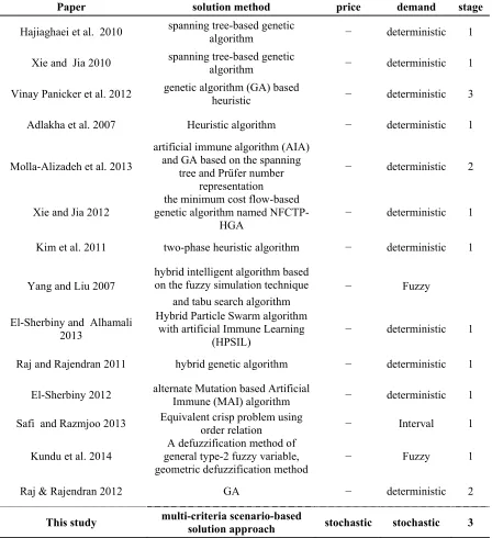
A defuzzification method of general type-2 fuzzy variable is outlined and compared numerically with geometric defuzzification method. Yang and Liu (Yang & Liu, 2007) investigate the fixed charge solid transportation problems under a fuzzy environment, in which the direct costs, the fixed charges, the supplies, the demand, and the conveyance capacities have been considered as fuzzy variables. They designed a hybrid intelligent algorithm based on the fuzzy simulation technique and tabu search algorithm to solve them. Table presents a review on some papers. The first row shows characteristics of this study. According to the above discussion, some gaps are considered in this paper:

 Most of the works in the literature consider the FCTP with deterministic parameters. Few works consider nondeterministic parameters, as seen in Table 1.

 Demand and transportation costs are considered under uncertainty (see Table 1). We consider price and demand in an uncertain environment.

 In nondeterministic works, fuzzy and interval are two main nondeterministic approaches. To the best of our knowledge we cannot find any papers with stochastic approach (about demand and price) in 3-stage supply chain.

(4)

Table 1: A review of planning under uncertainty for FCTP

Paper solution method price demand stage

Hajiaghaei et al. 2010 spanning tree-based genetic _algorithm − deterministic 1

Xie and Jia 2010 spanning tree-based genetic _algorithm − deterministic 1

Vinay Panicker et al. 2012 genetic algorithm (GA) based _heuristic − deterministic 3

Adlakha et al. 2007 Heuristic algorithm − deterministic 1

Molla-Alizadeh et al. 2013

artificial immune algorithm (AIA) and GA based on the spanning

tree and Prüfer number representation

− deterministic 2

Xie and Jia 2012

the minimum cost flow-based genetic algorithm named

NFCTP-HGA

− deterministic 1

Kim et al. 2011 two-phase heuristic algorithm − deterministic 1

Yang and Liu 2007

hybrid intelligent algorithm based

on the fuzzy simulation technique − Fuzzy and tabu search algorithm

El-Sherbiny and Alhamali 2013

Hybrid Particle Swarm algorithm with artificial Immune Learning

(HPSIL)

− deterministic 1

Raj and Rajendran 2011 hybrid genetic algorithm − deterministic 1

El-Sherbiny 2012 alternate Mutation based Artificial _{Immune (MAI) algorithm} − deterministic 1

Safi and Razmjoo 2013 Equivalent crisp problem using _{order relation} − Interval 1

Kundu et al. 2014

A defuzzification method of general type-2 fuzzy variable, geometric defuzzification method

− Fuzzy 1

Raj & Rajendran 2012 GA − deterministic 2

This study multi-criteria scenario-based _{solution approach} stochastic stochastic 3

3. Problem description

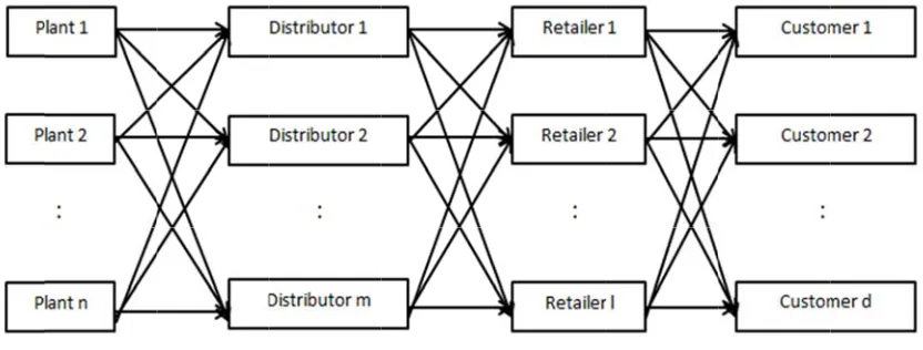
The presented three-stage fixed charge transportation problem includes n plants, m distributors, l retailers and d customers (see Figure 1). The characteristics of the model are as follows:

 The model is scenario-based. Demand and price are nondeterministic and it could be different for each scenario. Scenarios are created randomly in the three groups with poor, medium and high logic.

 The number and capacity of all facilities, and all cost parameters are predetermined.

(5)

 Each of the m distribution centres can ship products to any of the l retailers. In other words, a retailer can replenish the inventory from multiple distribution centres.

 Each of the n plants can ship products to any of the m distribution centres. In other words, a distribution centre can replenish the inventory from multiple plants.

 The production shortage is allowed. The backorder penalty cost is considered.

Notations are presented as follows: i: Set of plants (i =1 to n)

j: Set of distribution centres (j = 1 to m)

r: Set of retailers (r = 1 to l) K: Set of customers (k = 1 to d)

S: Demands and price scenarios (s = 1 to g)

ijs

x : Number of quantity transported from plant i to distributor j under scenario s.

ij

c : Unit cost of transportation between plant i and distributor j.

ij

f : Fixed transportation cost between plant i and distributor j.

jrs

u : Number of quantity transported from distributor j to retailer r under scenario s.

jr

b : Unit cost of transportation between distributor j and retailer r.

jr

o : Fixed transportation cost between distributor j and retailer r.

rks

t : Number of quantity transported from retailer r to customer k under scenario s.

rk

v : Unit cost of transportation between retailer r and customer k.

rk

q : Fixed transportation cost between retailer r and customer k.

ks

D : Demand at customer k under scenario s.

ks

P : Sales price at customer k under scenario s.

ks

H : Number of units backordered at customer k under scenario s.

k

Hc : Unit cost of backorder at customer k.

i

Am : Capacity at plant i.

j

Ad : Capacity at distributor j.

r

Ar : Capacity at retailer r.

ijs

z : Binary variable that specifies whether the product is distributed from plant i to distribution centre j under scenario s. (z_ijs= 0 or 1)

jrs

y : Binary variable that specifies whether the product is distributed from distribution center j to retailer r under scenario s. (y_jrs= 0 or 1)

rks

(6)

Journal o The fixe Maximi 1 1 1 g s k g d s k Z H     



Subject 1 m ijs j x  



1 n ijs i x  



1 m jrs j u  



1 l rks r t  



1 n ijs i x  



1 m jrs j u  



, , ijs jrs x u ijs ijs

z x

jrs j

y u

rks r

w t



0 ijs z 



0 jrs y 



0 rks w  The obj total co

of Industrial En

ed-charge tr ize: 1 1 g d ks ks k s ks k P D H Hc   



to: i Am  j Ad  r Ar 

0.8Dks

 1 l jrs r u  



1 d rks k t  



,t_rsk 0

s z Mijs jrs y Mjrs rksw Mrks



0,1



0,1



0,1 jective func sts. The tot

ngineering an

ransportatio



1 1 1

n m ij ijs i j c x  



i= 1, …

j = 1,

r = k = j = r = ( fo i = j= r= i= j= r= ction (1) is t tal cost is th

nd Managemen

Figure 1: P

on problem



1 g ij ijs s f z   



… , n

… , m

1, … , l

1, … , d

1, … , m

1, … , l

or all i, j, r, k = 1,…,n 1,…,m 1,…,l 1,…,n 1,…,m 1,…,l to maximiz he total cost

nt Studies (JIE

Proposed thre

is formulate



1 1 1

m l jr jr j r b u  



s = 1,… , g

s = 1, … ,

s = 1, …

s = 1,

k and s) j= 1,… r= 1,… k= 1,… j= 1,… r= 1,… k= 1, e the total p t transportat

N. Shira

EMS), Vol. 2,

ee-stage FCT

ed as follow



rso yjr jrs 

g

… , g

…,m …,l …,d …,m …,l ,…,d profits that tion incurre

azi, M. Seyyed

No. 1

TP.

ws:



1 1 1

g l d rk s r k

v    



s = 1, … , g s = 1, … , g s = 1, … ,

s = 1, … , g s = 1, … , g s = 1, … , is calculate ed in supply

d-Esfahani, H



k rkst q wrk rks

g g g g g , g ed by total s ying the pro

(7)

plants to customers through distributors and retailers, considering the possible combination of routes, plus shortage costs. Constraint (2) represents plant capacity constraint. This constraint maintains that the product quantity which is distributed from the plant to the distribution centers must be less than or equal to capacity of the plant. Constraint (3) denotes distributor capacity constraint. This constraint implies that the quantity of products received in a distribution center from plants must be less than or equal to the capacity of the distribution center. Constraint (4) indicates retailer capacity constraint. This constraint maintains that the quantity of products received in a retailer from distribution centers must be equal to or less than the capacity of the retailer. Constraint (5) denotes customer demand constraint. This constraint maintains that the retailers must provide at least 80 percent of customer’s demand. So, the shortage is allowed. Constraint (6) is the balance constraints of distributors. This maintains that all entering flows to a distribution center and all issuing flows from it are equal. Constraint (7) is the balance constraints of retailers. This constraint guarantees that all entering flows to a retailer and all issuing flows from it are equal. Constraint (8) ensures the non-negativity nature of decision variables. Constraint (9) to (14) asserts the 0–1 binary nature of the binary variable. These constraints maintain that if > 0, then =1, if > 0, then = 1 and if > 0, then

=1 .

4. Solution methodology

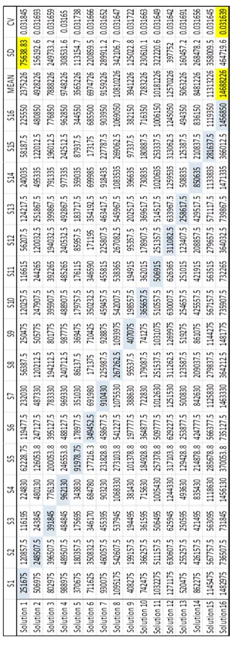
Scenario-based approaches for solving the stochastic programming problems are efficient methodologies (Kaut & Wallace, 2003; Listeş, 2007). In this paper, the problem is solved with using a multi criteria scenario based solution approach , that the first time is presented by Soleimani (Soleimani, Seyyed-Esfahani, & Shirazi, 2013). Mean, standard deviation and coefficient of variation, which are the mentioned criteria for finding the optimal solution.

The solution of this mathematical model consists of two plants, two distribution centers, two retailers and two customers. It is undertaken for two products and 16 scenarios. Then, 2 various possibilities for demands and prices based on the 4 range of the data in Table 2 are created randomly. A set of system’s parameters are presented in Table 3.

Table 2: Range of the demand and price in scenarios.

Low-quality Medium-quality High-quality Very High-quality

Demand 100─200 200─300 300─400 400─500

Price 10000─12000 12000─14000 14000─16000 16000─18000

Table 3: Parameters of the computational study

Parameter value

unit cost of transportation between plant i and distributor j ( ) = 100

= 200

(8)

= 300 = 100 = 200

fixed transportation cost between distributor j and retailer r( ) = 550

= 400 = 200 = 350

unit cost of transportation between retailer r and customer k ( ) = 300

= 150 = 200 = 200

fixed transportation cost between retailer r and customer k ( ) = 500

= 250 = 350 = 250

unit cost of backorder at customer k( ) = 10000

= 15000

capacity at plant I ( ) 500

capacity at distributor j ( ) 500

capacity at retailer r ( ) 500

The solution steps are illustrated as follows:

Step 1: all scenarios are solved by LINGO and the optimum points are obtained and recorded as candidate solutions for final optimal point. The results are illustrated in Table 4. Figure 2 presents the objective function values of 16 scenarios

Table 4: objective function values of 16 scenarios.

Scenarios S1 S2 S3 S4 S5 S6 S7 S8

Profit 251675 248507.5 391845 962130 91978.75 349452.5 910430 2.67E+05

Scenarios S9 S10 S11 S12 S13 S14 S15 S16

(9)

 Step sce 6 sc 0.02 wit ans  Step sce eva the valu sce  Step acc crit and  Step sen app

p 2: scenar narios with cenarios wi 25. The pro th high logi swers are ca p 3: the in narios and aluated in 1 performan ues). Then, narios. The p 4: We us ceptable crit teria of mak d 5).

p 5: optima nsitivity ana

proach.

Figu

rios in the t h poor logic ith high log obability of

ic is 0.1 .A alculated wi

nitial respo objective fu 6 different ces of a ca , weighted results are sed three cr teria to sel king final d

al solution alyses are u

ure 2: Objecti

three group have 0.5w gic have 2w f scenarios w After obtain

th using the onse of 16 function val scenarios s andidate sol average of presented i riteria (mea ect the bes decision of t

is selected undertaken

ive function v

ps with poo weight. 6 s weight. Th with medium ning the an e probability

scenarios lues are rec so the mode lution are ev f answers is

n Table 5. an, standard st solution. the best sol

based on th to determin

values of 16 s

or, medium scenarios w he probabili m logic is 0 nswer of 16 y of scenari (candidate corded. We el should b

valuated in s calculated

d deviation The last th lution in va

he analyses ne the relia

scenarios

and high l with medium

ity of scena 0.05. The pr 6 scenarios, ios.

solutions) have 16 so e solved 25 n 16 scenari d according

, and coeff hree column arious situat

s of three cr ability of th

logic are cl m logic have

arios with po robability o , weighted

are evalu olutions that

56 times. In ios (objectiv g to the pro

ficient of va ns of Table tions (see F

riteria and he develope

assified. 4 e w weight. oor logic is of scenarios average of

uated in all t should be n each row, ve function obability of

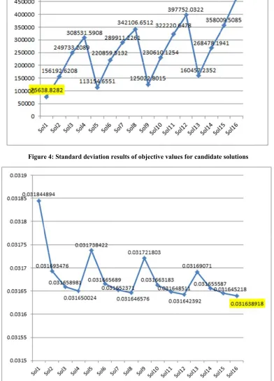
ariation) as e 5 are the Figures 3, 4

(10)

Journal oof Industrial Enngineering an

T

ab

le 5:

Scenari

o-b

ased

solu

tion

app

roac

h

for

stoc

h

astic mod

el

nd Managemennt Studies (JIE

N. Shira

EMS), Vol. 2,

azi, M. Seyyed

No. 1

d-Esfahani, HH. Soleimani

Page 36

i

(11)

We ana discusse The me This va solution Mean c uncertai decision variance fluctuat Table 5 So, it ca there ar approac solution

alyzed Tabl ed as follow ean objectiv

lue is maxi n. It is illustr

riteria is no in situation ns of deci e) as risk c ted environm

and Figure an be select re two diffe ch to make ns. It can be

le 5 and F ws:

ve function v mum profit rated in Fig ot enough f ns there are sion maker criterion. E ment. SD i e 4. Accord ted as more erent optim e final dec selected as

Figure 3:

Figures 3, 4

value of sol t mean amo gure 3.

for selecting e fluctuation rs (Ogrycz Each of the s achieved ding to the T e reliable in mal solutions

ision. Solu s the final op

Mean results

4, and 5 fo

lution 16 th ong all solut

g optimal so ns and we zak, 2000).

solutions for all solu Table 5 and n uncertain c s. We can u ution 16 ha

ptimal solut

s of objective

for finding

hat is obtain tions. So, w

olution. Be need a risk We cons that have l utions of sc d Figure 4, conditions. use coeffici as the min

tion. It is pr

e values for ca

the optima

ned by scen we can selec

ecause in di k criteria to ider standa lower SD, cenarios. Re

solution 1 Regarding ient of vari nimum CV

resented in F

andidate solu

al solution,

nario 16 , is ct it as best

fferent con o ensure re ard deviati

it is more esults are p

has the min mean and S iation as an

(12)

Journal o

5. Co

In this formula

of Industrial En

Figur

Figure 5

onclusion

paper, is c ated as a mix

ngineering an

e 4: Standard

5: Coefficient

and futu

considered

xed integer

nd Managemen

d deviation re

t of variation

re researc

a three-stag programmi

nt Studies (JIE

esults of obje

n results of ob

ches

ge fixed ch ing problem

N. Shira

EMS), Vol. 2,

ective values f

bjective value

harge transp m and is solv

azi, M. Seyyed

No. 1

for candidate

es for candida

portation pr ved using a

d-Esfahani, H

e solutions

ate solutions

roblem. Th multi-criter

H. Soleimani

Page 38

he model is ria scenario i

8

(13)

based solution approach to find optimal solution. First,16 scenarios with different logical are generated randomly. Then, initial solutions of scenarios are evaluated and weighted average of the results is calculated. Finally, mean, standard deviation and coefficient of variation are regarded as acceptable criteria in order to decide about best solution. This model can be expanded to a multi-product and multi-period for the future research.

References

1. Adlakha V., Kowalski, K. 1999. “On the fixed-charge transportation problem”. Omega, 27(3),

381-388.

2. Adlakha V., Kowalski, K. 2010. “A heuristic algorithm for the fixed charge problem”. Opsearch, 47(2), 166-175.

3. Adlakha V., Kowalski K., Lev B. 2010. “A branching method for the fixed charge transportation problem”. Omega, 38(5), 393-397.

4. Adlakha V., Kowalski K., Vemuganti R. R., Lev B. 2007. “More-for-less algorithm for fixed-charge transportation problems”. Omega, 35(1), 116-127.

5. Adlakha V., Kowalski K., Wang S., Lev B., Shen W. 2014. “On approximation of the fixed charge transportation problem”. Omega, 43(0), 64-70.

6. Antony Arokia Durai Raj K., Chandrasekharan R. 2012. “A genetic algorithm for solving the fixed-charge transportation model: Two-stage problem”. Computers & Operations Research, 39(9),

2016-2032.

7. Balinski, Michel L. 1961. “Fixed‐cost transportation problems”. Naval Research Logistics Quarterly, 8(1), 41-54.

8. Diaby, Moustapha. 1991. “Successive linear approximation procedure for generalized fixed-charge transportation problems”. Journal of the Operational Research Society, 991-1001.

9. El-Sherbiny, Mahmoud M., Alhamali, Rashid M. 2013. “A hybrid particle swarm algorithm with artificial immune learning for solving the fixed charge transportation problem”. Computers & Industrial Engineering, 64(2), 610-620.

10. El-Sherbiny, M.M.. 2012. “Alternate mutation based artificial immune algorithm for step fixed charge transportation problem”. Egyptian Informatics Journal, 13(2), 123-134.

11. Eskigun E., Uzsoy R., Preckel P.V., Beaujon G., Krishnan S., Tew J. D. 2005. “Outbound supply chain network design with mode selection, lead times and capacitated vehicle distribution centers”.

European Journal of Operational Research, 165(1), 182-206.

12. Gen, M., Kumar A., Ryul Kim J. 2005. “Recent network design techniques using evolutionary algorithms”. International Journal of Production Economics, 98(2), 251-261.

13. Hajiaghaei-Keshteli M., Molla-Alizadeh-Zavardehi, S., Tavakkoli-Moghaddam, R. 2010. “Addressing a nonlinear fixed-charge transportation problem using a spanning tree-based genetic algorithm”. Computers & Industrial Engineering, 59(2), 259-271.

14. Hitchcock, F.L. 1941. “The distribution of a product from several sources to numerous localities”. J. Math. Phys, 20(2), 224-230.

15. Jawahar, N, & Balaji, AN. 2009. “A genetic algorithm for the two-stage supply chain distribution problem associated with a fixed charge”. European Journal of Operational Research, 194(2),

496-537.

(14)

21. Listeş O. 2007. “A generic stochastic model for supply-and-return network design”. Computers & Operations Research, 34(2), 417-442.

22. Lotfi, M. M., & Tavakkoli-Moghaddam, R. 2013. “A genetic algorithm using priority-based encoding with new operators for fixed charge transportation problems”. Applied Soft Computing, 13(5), 2711-2726.

23. Molla-Alizadeh-Zavardehi, S., Sadi Nezhad, S., Tavakkoli-Moghaddam, R., & Yazdani, M. 2013. “Solving a fuzzy fixed charge solid transportation problem by metaheuristics”. Mathematical and Computer Modelling, 57(5–6), 1543-1558.

24. Ogryczak, W. 2000. “Multiple criteria linear programming model for portfolio selection”. Annals of Operations Research, 97(1-4), 143-162.

25. Panicker, V.V., Sridharan R., Ebenezer B. 2012. “Three-stage supply chain allocation with fixed cost”. Journal of Manufacturing Technology Management, 23(7), 853-868.

26. Pintea C.M., Sitar C., Hajdu-Macelaru M., Petrica P. 2012. “A Hybrid Classical Approach to a Fixed-Charged Transportation Problem. Hybrid Artificial Intelligent Systems, 7208, 557-566.

27. Raj, K Antony Arokia Durai, & Rajendran, Chandrasekharan. 2011. “A Hybrid Genetic Algorithm for Solving Single-Stage Fixed-Charge Transportation Problems”. Technology Operation Management, 2(1), 1-15.

28. Safi, M. R., & Razmjoo, A. 2013. “Solving fixed charge transportation problem with interval parameters”. Applied Mathematical Modelling, 37(18–19), 8341-8347.

29. Schaffer, Joanne R, & O'Leary, Daniel E. 1989. “Use of penalties in a branch and bound procedure for the fixed charge transportation problem”. European journal of operational research, 43(3),

305-312.

30. Soleimani H., Seyyed-Esfahani M., Shirazi M. 2013. “A new multi-criteria scenario-based solution approach for stochastic forward/reverse supply chain network design”. Annals of Operations Research, 1-23.

31. Vinay, VP, Sridharan, R. 2012. “Development and analysis of heuristic algorithms for a two–stage supply chain allocation problem with a fixed transportation cost”. International Journal of Services and Operations Management, 12(2), 244-268.

32. Xie F., Jia R. 2010. “A note on “Nonlinear fixed charge transportation problem by spanning tree-based genetic algorithm”, Computers & Industrial Engineering, 59(4), 1013-1014.

33. Xie F., Jia R. 2012. “Nonlinear fixed charge transportation problem by minimum cost flow-based genetic algorithm”. Computers & Industrial Engineering, 63(4), 763-778.