Simulation of the time-variable gravity field by means of coupled geophysical models

Earth Syst. Sci. Data, 3, 19–35, 2011 www.earth-syst-sci-data.net/3/19/2011/ doi:10.5194/essd-3-19-2011

©Author(s) 2011. CC Attribution 3.0 License.

History

Geo- and Space

Sciences

Open

Access

Advances

Open Access Proceedings

Open

Access

Earth System

Science

Data

Access

Earth System

Science

Data

D

iscussions

Drinking Water

Open Access

Drinking Water

Discussions

O

pen

Acc

es

s

Social

Geography

Open

Access

D

iscussions

Social

Geography

Open

Access

Simulation of the time-variable gravity field by means of

coupled geophysical models

Th. Gruber1_{, J. L. Bamber}2_{, M. F. P. Bierkens}3_{, H. Dobslaw}4_{, M. Murb¨ock}1_{, M. Thomas}4_,

L. P. H. van Beek3, T. van Dam5, L. L. A. Vermeersen6, and P. N. A. M. Visser6

1_{Institute of Astronomical and Physical Geodesy, Technical University Munich, Munich, Germany} 2_{Bristol Glaciology Centre, University of Bristol, Bristol, UK}

3_{Department of Physical Geography, Utrecht University, Utrecht, The Netherlands} 4_{Deutsches GeoForschungsZentrum Potsdam, Potsdam, Germany}

5_{University of Luxembourg, Luxembourg}

6_{Delft Institute of Earth Observation and Space Systems, Delft University of Technology, Delft,} The Netherlands

Received: 7 June 2011 – Published in Earth Syst. Sci. Data Discuss.: 7 July 2011 Revised: 6 October 2011 – Accepted: 7 October 2011 – Published: 31 October 2011

Abstract. Time variable gravity fields, reflecting variations of mass distribution in the system Earth is one of the key parameters to understand the changing Earth. Mass variations are caused either by redistribution of mass in, on or above the Earth’s surface or by geophysical processes in the Earth’s interior. The first set of observations of monthly variations of the Earth gravity field was provided by the US/German GRACE satellite mission beginning in 2002. This mission is still providing valuable information to the science community. However, as GRACE has outlived its expected lifetime, the geoscience community is currently seeking suc-cessor missions in order to maintain the long time series of climate change that was begun by GRACE. Several studies on science requirements and technical feasibility have been conducted in the recent years. These studies required a realistic model of the time variable gravity field in order to perform simulation studies on sensitivity of satellites and their instrumentation. This was the primary reason for the European Space Agency (ESA) to initiate a study on “Monitoring and Modelling individual Sources of Mass Distribution and Transport in the Earth System by Means of Satellites”. The goal of this interdisciplinary study was to create as realistic as possible simulated time variable gravity fields based on coupled geophysical models, which could be used in the simulation processes in a controlled environment. For this purpose global atmosphere, ocean, continental hydrology and ice models were used. The coupling was performed by using consistent forcing throughout the models and by including water flow between the different domains of the Earth system. In addition gravity field changes due to solid Earth processes like continuous glacial isostatic adjustment (GIA) and a sudden earth-quake with co-seismic and post-seismic signals were modelled. All individual model results were combined and converted to gravity field spherical harmonic series, which is the quantity commonly used to describe the Earth’s global gravity field. The result of this study is a twelve-year time-series of 6-hourly time variable gravity field spherical harmonics up to degree and order 180 corresponding to a global spatial resolution of 1 degree in latitude and longitude. In this paper, we outline the input data sets and the process of combining these data sets into a coherent model of temporal gravity field changes. The resulting time series was used in some follow-on studies and is available to anybody interested.

1 Introduction

The primary goal of the recently completed European Space Agency (ESA) study entitled “Monitoring and Modelling

in-Correspondence to: Th. Gruber

([email protected])

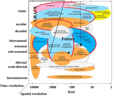
Figure 1.Time variable gravity field sources in terms of spatial resolution and time variability including GRACE sensitivity and goals for future gravity field missions.

the solid Earth and environmental surface processes within the Earth’s outer fluid envelop (excluding tides). It shall be noted that “realistic” is understood in the sense that all spec-tra of variability shall be included in a comprehensive time-variable gravity field model in order to perform simulations approximating reality. A simulation time period of 12 yr spanning the years 1995 to 2006 was chosen. The resulting predictive model of the time variable gravity field is unique in the sense of signal sources incorporated, coupling of geo-physical models and a decadal simulation period. No similar data sets have been published yet in the geoscience commu-nity. Here, we address the development of the realistic Earth model, which is described in detail below. The second step was to use the realistic Earth mass model to develop satellite orbits and configurations to monitor the changes such that we are able to separate the different components of the mass variability. The twin-satellite GRACE mission has shown that time variable gravity field is observable from space on a monthly base with spatial resolutions of a few hundred kilo-metres (Tapley et al., 2004). GRACE observes inter-satellite distance changes with a fewµm accuracy, which are caused to a large extent by irregularities of the mass distribution in,

on or above the Earth. Studies on future gravity field mission constellations target on higher temporal and spatial resolu-tion by enhancing the observaresolu-tion accuracy and/or by im-plementing new satellite configurations. The subsequent re-search in which different satellite orbits and configurations were tested has already been described in Visser et al. (2010). An overview of time variable gravity field sources in terms of spatial resolution and time variability is shown in Fig. 1. The horizontal axis defines the spatial resolution, while the vertical axis specifies the time variability from instantaneous to static. The bubbles define signals from various sources and their estimated space-time variability. The colours of the bubbles classify the sources for different domains. In addition the box identifies, what signals are sensitive to the GRACE mission (see below). The two dotted lines indicate somehow the signals to be observable by future gravity field missions, without specifying the requirements in detail.

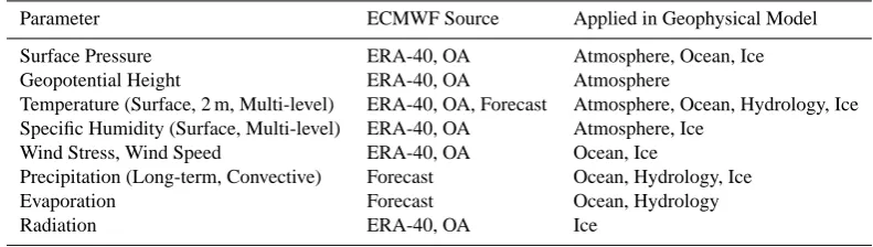
Table 1.Atmospheric parameters from ECMWF used for this study (ERA-40=Reanalysis, OA=Operational Analysis). Parameter ECMWF Source Applied in Geophysical Model Surface Pressure ERA-40, OA Atmosphere, Ocean, Ice Geopotential Height ERA-40, OA Atmosphere

Temperature (Surface, 2 m, Multi-level) ERA-40, OA, Forecast Atmosphere, Ocean, Hydrology, Ice Specific Humidity (Surface, Multi-level) ERA-40, OA Atmosphere, Ice

Wind Stress, Wind Speed ERA-40, OA Ocean, Ice

Precipitation (Long-term, Convective) Forecast Ocean, Hydrology, Ice Evaporation Forecast Ocean, Hydrology Radiation ERA-40, OA Ice

effect of the mass distribution at a specific time, simulating the time variable gravity field from the separate geophysical models needs to be made consistent and the models need to be coupled. Consistency means that geophysical model re-sults need to be converted, such that they provide the same quantity for mass distribution at a specific time (e.g. pres-sure, equivalent water height or gravitational attraction), that the geospatial sampling is identical (e.g. geographical grid) and that they all refer to the same reference values (e.g. a mean field). The procedure applied to secure consistency is described in some detail in Sect. 7. More important, how-ever, is the coupling of the geophysical models that together define the water cycle. For a realistic Earth model, we need to insure that mass flowing from one component to the other domain is not “lost” in the system or conversely that it is not counted twice.

The coupling was performed by imposing that the forcing data be consistent over all models, i.e. all our surface mass models use forcing parameters from the same source (in our case the ECMWF atmospheric model) (see Sect. 2) and that water flowing from the continents (including continental ice) to the oceans is taken into consideration by the models. By using an identical forcing model, we guarantee that water ex-change between the atmosphere and the Earth surface (con-tinents and oceans) is taken into account intrinsically.

For coupling the geophysical models on the ground, spe-cific adaptations were made, including the harmonization of land/ocean masks and the provision of outgoing water mass from one domain to another. Detailed descriptions of the geophysical models and the adaptations made for coupling them are provided in Sects. 3–5 for the continental hydrol-ogy, the continental ice and the ocean, respectively.

For the solid Earth processes, global isostatic adjustment was included as a continuous process and an earthquake as a sudden event. Their predicted impact on the gravity field was taken into account. Details on this aspect of the modelling will be provided in Sect. 6. Finally, Sect. 8 summarizes the work performed and provides some conclusions to be drawn from the results obtained.

2 Atmosphere

The atmosphere is one of the main contributors to mass vari-ations in the Earth system. Atmospheric mass varivari-ations are present for periods ranging from a few hours to decadal. The primary manifestation of atmospheric mass variations, are the distribution and propagation of the pressure systems around the globe. However high frequency mass variability also occurs in the form of diurnal and the semi-diurnal atmo-spheric tides.

For modelling the atmospheric mass variations as well as for forcing the geophysical models, a global atmospheric model was applied. For this study we used the operational, the re-analysis (ERA-40) and the related short-term forecast models driven by the European Centre for Medium-Range Weather Forecasts (ECMWF). The latter model needs to be used for some parameters not available in the other two model versions. In order to identify the impact of using at-mospheric data with different consistency over time, we used atmospheric parameters from the operational and the reanal-ysis model for different periods. Reanalysis data (ERA-40) were used for the years 1995 to 1999, while for the time span from 2000 until 2006 data from the ECMWF opera-tional analysis were used. The list of atmospheric parameters and the geophysical models for which they are subsequently used is provided in Table 1. In general, we used the 6-hourly time series of the atmospheric parameters indicated. All at-mospheric parameters were extracted from the ECMWF data base according to the requirements of the geophysical mod-els. More details about the hydrology, ocean and continental ice models are provided in the subsequent Sects. 3 to 5.

For the atmospheric mass distribution per time step, the required parameters were extracted as 1×1◦ _equi-angular

satellite orbits and configurations one would need in addi-tion the geopotential surface and the multi-layer atmospheric temperature and specific humidity data. For the combination of the different mass fields as described in Sect. 7 we finally have available 6 hourly surface pressure grids in units of Pas-cal from the ERA-40 reanalysis model (for the years 1995 to 1999) and from the operational analysis (for years 2000 to 2006).

3 Continental hydrology

We used the global hydrological model PCR-GLOBWB (Van Beek and Bierkens, 2009; Bierkens and Van Beek, 2009) to estimate terrestrial water storage anomalies. PCR-GLOBWB calculates for each grid cell (0.5×0.5◦_globally)

and for each time step (daily) the water storage in two ver-tically stacked soil layers and an underlying groundwater layer, as well as the water exchange between the layers and between the top layer and the atmosphere (rainfall, evapo-ration and snow melt). The model also calculates canopy interception and snow storage. Sub-grid variability is taken into account by considering separately tall and short vege-tation, open water, different soil types and the area fraction of saturated soil and the frequency distribution of ground-water depth based on the surface elevations of the 1×1 km Hydro1k data set. Fluxes between the lower soil reservoir and the groundwater reservoir are mostly downward, except for areas with shallow groundwater tables, where fluxes from the groundwater reservoir to the soil reservoirs are possible (i.e. capillary rise) during periods of low soil moisture con-tent. The total specific runoffof a cell consists of satura-tion excess surface runoff, melt water that does not infiltrate, runofffrom the second soil reservoir (interflow) and ground-water runoff(baseflow) from the lowest reservoir. To cal-culate river discharge, specific runoffis accumulated along the drainage network by means of kinematic wave routing including storage effects and evaporative losses from lakes, reservoirs and wetlands.

3.1 Adaptation of model made for this study

Forward modelling with PCR-GLOBWB returned daily fields of terrestrial freshwater storage with a resolution of 0.5◦ for the period 1957–2006. The model was forced with ECMWF meteorological data for precipitation, air tempera-ture and actual evaporation. For the period 1957–1999 in-clusive, daily surface fields were obtained from ERA-40 re-analysis forecasts, from 2000 onwards from forecasts of the Operational Archive. To preserve consistency in the meteo-rological forcing, actual evaporation from the ECMWF fore-casts was imposed directly on the model and partitioned over the different surface areas within each cell on the basis of cover fraction. Following the parameterization of the model, bare soil evaporation was drawn from the upper soil layer whereas transpiration by vegetation was broken down over

both soil layers on the basis of root fractions. The imposed evaporative flux was not reduced, unless the absolute soil wa-ter storage was insufficient to sustain it.

Since glacier melt has only limited influence on discharge, glacier dynamics were insufficiently represented in PCR-GLOBWB to resolve variations in water storage over this type of terrain realistically. To amend this, four regions with significant terrestrial glacier mass were included separately in the model in addition to the land ice masses of Greenland and Antarctica, which were modelled separately by BGC (see below). The melt of the land ice mass of Greenland and Antarctica was supposed to drain directly to the ocean and the corresponding areas masked out. For the four glaciated regions (Alaska, Alps, Karakoram, and Himalayas), melt contributes to streamflow in PCR-GLOBWB. Glacier melt was assumed to follow a secular trend of 1 % per year from 1990 onwards starting with initial volumes of 7500, 1500, 4000 and 4000 km3_{for the respective areas (J. Bamber,} per-sonal communication, 2008). To obtain a finer representation of glaciers in these regions, the glacier volumes were down-scaled proportional to the glacier coverage within each 0.5◦

cell as represented by the FAO digital soil map of the world (FAO, 2011). At the beginning of 1990, the glacier volumes in these four regions were initialized at the estimated vol-umes, with variations arising due to precipitation and evap-oration over time, and the secular melt rate applied. This melt rate was further broken down into monthly values on the basis of the temperature climatology of the ERA-40 dataset with the melt rate being proportional to the deviation above the mean annual temperature. Prior to this date, the melt rate was assumed to be zero for these four regions. An additional problem was encountered in those areas where the long-term temperature of the EMCWF data did not exceed 0◦_{C and}

that were not identified as glaciated areas a priori. The cor-responding cells were identified entirely as glaciers and the mass balance of precipitation, evaporation and glacier melt evaluated with the latter amounting to 100 % of the accumu-lated volume per year.

Figure 2. Cumulative, area-averaged trend in ECMWF forcing (precipitation minus actual evaporation) over endorheic basins, per continent and for the Caspian Sea and Aral Sea. South America, gaining 8.7 m over the entire period, is not shown.

3.2 Description of resulting hydrology mass fields

Including the glaciated areas, anomalies in the hydrology mass fields represent the seasonal and inter-annual variations realistically over large areas. Small inconsistencies arise due to the fact that the spatial resolution of the ECMWF forc-ing is finer for the Operational Archive than for the ERA-40 reanalysis; at these transitions abrupt changes in the to-pographic effect on temperature leads to sudden snow melt and variations in the available storage. Overall, however, the quality of the hydrology mass fields is good over the North-ern Hemisphere where the forecasts are well constrained by meteorological information, the amount of precipitation is large, and the resulting conversion into runoffis not unduly influenced by model errors. Elsewhere the quality can be affected by a poorer meteorological forcing and by biased and uncertain variables and unresolved processes (e.g. sim-ple representation of snow and glacier melt). In addition, the ERA-40 reanalysis demonstrates variable skill in predict-ing precipitation for different zones and for different peri-ods (Troccoli and Kållberg, 2004) and its water balance not closed. Particularly troubling are the long-term trends over the 14 % of the terrestrial surface that has no direct link to the oceans. Such endorheic basins are particularly sensitive to small variations in evaporative losses (and errors therein) as the accumulated runoffcan only be lost to the atmosphere. Thus, gains or losses over these areas will directly affect the simulated storage (Fig. 2).

Negative fluxes over North America and Europe are rela-tively small when the corresponding area is taken into con-sideration. They are more substantial for the arid conti-nents of Australia and Africa over the simulation period but in these water-limited environments this will not have large

repercussions on the total storage. Where the trends are pos-itive, for example for the Caspian Sea and Asia, the accu-mulations are significant as these areas correspond to 10 % of the total terrestrial land mass. For the Caspian Sea, the increases from the mid-1990s onwards can be linked to in-creased discharge from the Volga due to a stronger North At-lantic Oscillation (NAO) and should not be discredited as a mere model artefact.

For South America, however, the strong positive trend is erroneous. In this study, such spurious trends in water stor-age have been removed from the hydrology mass storstor-age fields as a post-processing step. Yet, drawing from the expe-rience of this study it would be advisable to force the model with a more consistent meteorological dataset and to im-pose reference potential evaporation. For each surface within PCR-GLOBWB, the specific potential evaporation can then be calculated using correction factors (or crop factors) (Allen et al., 1998) and scaled to the actual rate on the basis of wa-ter availability within the hydrological model. Tuning of the correction factors can then reduce spurious long-term trends. Although the a posteriori removal of trends largely resorts in the same effect, tuning the correction factors is slightly more transparent and may preserve regional and temporal detail that is currently lost.

4 Ice

4.1 Background

The purpose of the ice mass flux models was not to, necessar-ily, reproduce the observed mass trends but to simulate real-istic seasonal and secular behaviour. The primary focus was on the contribution of the two largest ice masses: the Green-land and Antarctic ice sheets (GrIS, AIS) in terms of for-ward modelling. For four glacierized regions, the European Alps, Himalaya, Karakoram and Gulf of Alaska (Fig. 4), we prescribed plausible secular mass loss trends that covered a range of signal magnitude from ∼15 to 75 Gt yr−1_{. These} fluxes were subsequently incorporated into the global hydrol-ogy model (see Sect. 3). In the rest of this Section we focus on how the ice sheet fluxes were prescribed.

Two processes that have different spatial and temporal be-haviours control the ice sheet fluxes: surface mass balance (SMB) and ice dynamics (ID). The former is determined by the balance between solid precipitation and runoff and re-sponds almost instantaneously to changes in external forc-ing. Inter-annual variability in SMB is large compared to, for example, secular trends in mass loss and it is important, therefore, that this is adequately simulated in addition to any underlying trends.

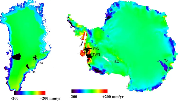
Figure 3. Left: surface mass deviation from an 11 yr mean for Greenland. The year shown here is 2000. JI=Jakobshavn Isbrae, Ka=Kangerdlugssuaq, He=Helheim. A negative trend in ablation was imposed starting in 2000 and is apparent around the margins. Right: as for a, but for Antartica. In this case, all deviations from the mean are due to inter-annual variability in snowfall except for ice dynamic losses for the glaciers that are labeled. PIG=Pine Island Glacier, TWG=Thwaites Glacier, ISC=Ice Stream C, To=Totten Glacier.

Figure 4. Location of four mountain glacier regions where a secular trend of 1 % of the total mass was imposed for the 11 yr of the hydrological model simulation.

resolution (both in time and space) gravity data and our aim was, therefore, to ensure that both these signals were realis-tically simulated to explore this issue.

4.2 Short description of the model and adaptation to the study

For the ice sheets, a time series of surface mass bal-ance fluxes were calculated for the period 1995–2005 using ECMWF reanalysis data (ERA-40 up to 2001) and the oper-ational analysis beyond. The data were produced on a 5 km polar stereographic grid with 6-hourly time step for

Figure 5.Daily mass trends integrated over the whole of the Green-land ice sheet. The values include both SMB and ice discharge.

signals but are also designed to capture a range of signal am-plitudes and spatial scales. An example of the deviation of the year 2000 SMB from the eleven-year mean is shown in Fig. 3, which also indicates the pattern of ice dynamic losses imposed for both ice sheets. The areas shaded black indicate regions where a secular trend in ice dynamics was imposed based on the 50 m a−1velocity contour for the outlet glacier. The spatial pattern and magnitude of the trends are compa-rable with recent observations of regional mass loss from, for example, SAR interferometry. In addition to the spatially distributed mass changes over the ice sheets we also calcu-lated the flux of ice at the margins entering the ocean grid cells. This was done with the aid of the OMCT ocean/land mask. For Antarctica the fluxes were calculated annually as there is no seasonal or daily variation so that the daily value was 1/365 of the annual value. For Greenland the margin fluxes were calculated on a daily time step due the seasonal-ity of surface runoff(cf. Fig. 5). Both Greenland and Antarc-tica were excluded from the hydrology model as explained in Sect. 3.

4.3 Description of resulting Greenland and Antarctic ice mass fields

The daily mass trends integrated over the whole of the Green-land Ice Sheet are shown in Fig. 5 starting on 1 January 1995. Positive values indicate snowfall and an increase in SMB that is evident in winter and spring. During summer, surface ab-lation dominates and results in a negative SMB. The mean is less than zero even when there is no surface ablation due to continuous solid ice discharge, which was assumed to have no significant seasonality.

The cumulative mass trends are shown in Fig. 6 and in-dicate the amplitude of the seasonal cycle in SMB which is around 300 Gt and is in good agreement with results from

Figure 6.Cumulative mass trends for the Greenland ice sheet.

Figure 7. Annual components (SMB and discharge) of the mass flux for Antarctica. Note the linear increase in discharge due to the effect of ice dynamic changes imposed. The right hand axis shows the net mass trend (SMB-discharge) for the whole ice sheet (green line).

GRACE (Van den Broeke et al., 2009). Starting at about day 1000, we imposed an increase in ice discharge and ablation that results in a roughly constant loss of mass to the oceans of 110 Gt a−1_{. This rate is comparable with mass balance} esti-mates of the ice sheet between the mid 1990s and mid 2000s (Van den Broeke et al., 2009). The spatial pattern of loss is distributed between increased runoffand discharge as shown in Fig. 3 left.

glaciers in Fig. 3 right) from 1995–2000 and then kept con-stant thereafter. The total increase was 100 Gt over the five year period (Fig. 7). This results in both negative and positive balance years depending on the snowfall in a particular year. The mass loss for the whole ice sheet is somewhat smaller than recent observations suggest (Velicogna, 2009) but the spatial distribution and magnitude of dynamic losses in the Amundsen Sea sector are quite close to observations (Rignot et al., 2008).

5 Ocean

The global Ocean Model for Circulation and Tides (OMCT) (Thomas, 2002) has been developed by adjusting the origi-nal climatological Hamburg Ocean Primitive Equation model (HOPE; Wolff et al., 1996; Drijfhout et al., 1996) to the weather time scale and coupling with an ephemeral tidal model. OMCT has been used to investigate the impact of the general ocean circulation on the Earth’s rotation and the gravity field (Thomas et al., 2001; W¨unsch et al., 2001; Dob-slaw and Thomas, 2005, 2007b) and is currently applied to de-alias short-term ocean mass anomalies within the GRACE gravity field processing (Flechtner, 2007).

The model is based on non-linear balance equations for momentum, the continuity equation, and conservation equa-tions for heat and salt. The hydrostatic and the Boussi-nesq approximations are applied. Water elevations, three-dimensional horizontal velocities, potential temperature as well as salinity are calculated prognostically, vertical veloci-ties are determined diagnostically from the incompressibility condition. Implemented is a prognostic thermodynamic sea-ice model (Hibler III, 1979) that predicts sea-ice-thickness, com-pactness and drift. Effects of loading and self-attraction of the water column are parameterized by means of a secondary potential proportional to the mass of the local water column (Thomas et al., 2001). The model uses a time-step of 30 min, a constant horizontal resolution of 1.875◦ _{in longitude and}

latitude, and 13 layers exist in the vertical.

A quasi steady-state circulation has been obtained from an initial model spun up for 265 yr using climatological wind stresses (Hellerman and Rosenstein, 1983) and mean sea surface temperatures and salinities according to Levi-tus (1982). Subsequently, OMCT has been forced by 6-hourly wind stresses, atmospheric surface pressure, 2 m tem-peratures and freshwater fluxes due to precipitation, evapo-ration and runoffobtained from the latest reanalysis project ERA-40 of the European Centre for Medium Range Weather Forecasts (ECMWF), and the Hydrological Discharge Model HDM (Walter, 2007) for the period 1958–1989. The fol-lowing 5 yr have been simulated using ERA-40 atmospheric data accompanied with climatologically averaged ice-sheet discharges (Sect. 4) and daily continental runoff(Sect. 3) in order to prevent numerical shocks due to sudden changes in forcing conditions. The period relevant for the data-set

described here, i.e. 1995 until 2006 has been simulated by applying forcing based on ERA-40 (1995–1999) and opera-tional ECMWF atmospheric data (2000–2006) together with daily discharges from continental hydrology (see Sect. 3), daily discharges from the Greenland ice-sheet, and annual ice discharges from Antarctica (Sect. 4).

Total ocean mass variations due to freshwater fluxes are considered up to seasonal time-scales. However, as sug-gested by Greatbatch (1994), artificial mass variations caused by the applied Boussinesq approximation have been cor-rected for (cf. Dobslaw and Thomas, 2007a). Oceanic mass fields have been stored every 6-h.

Ocean mass anomalies have been obtained by reducing the mean field averaged over 2000–2005. Due to the shift in atmospheric forcing conditions from ERA-40 towards op-erational ECMWF analyses in 2000, mean atmosphere and ocean mass fields change at this time substantially, as can be deduced from the differences of mean atmospheric pres-sure as well as ocean mass for the periods 1995 until 1999 and 2000 until 2005 (Fig. 8). Differences over continental regions are mainly due to the improved spatial resolution in the operational model, allowing a more detailed representa-tion of the orography. The largest deviarepresenta-tions over the oceans occur mainly in coastal regions, which are both related to artifacts caused by the required horizontal interpolation to-wards the OMCT grid as well as to the different spatial res-olution. However, large-scale differences with small but still relevant amplitudes exist in the open ocean, e.g. in the south-ern Pacific, which might lead to systematic biases. In order to remove this bias as much as possible, a mean field for the ERA-40 period has been calculated by minimising the diff er-ences between mass anomalies from simulations forced by ERA-40 and the operational ECMWF data in the overlap-ping years 2000 and 2001, separately for atmospheric and oceanic mass anomalies. The obtained mean field has been removed from all ERA-40 forced data covering 1995–1999.

Variability of regional ocean mass anomalies is essen-tially comparable in the run analysed in Dobslaw and Thomas (2007a). The highest variability occurs in the South-ern Oceans as well as in the North Pacific, and, with slightly smaller amplitudes, in the Arctic basin. Small scale sig-nals with significantly higher amplitudes additionally occur in various shelf regions but are generally less reliable due to the 1.875◦horizontal resolution of the OMCT. While vari-ability is fairly comparable for both simulated periods, appar-ent bottom pressure trends alter significantly when changing from ERA-40 to operational ECMWF forcing fields (Fig. 9). At this point, causes for these apparent changes in the trends are not clear and remain the subject for further studies.

Figure 8.Differences of mean mass fields [hPa] calculated for (a) atmospheric pressure and (b) ocean water mass between the time periods 1995–1999 and 2000–2005, respectively.

Figure 9.Trends in ocean bottom pressure as derived for (a) the period 1995–1999 forced by ERA-40 and (b) the period 2000–2005 forced by operational ECMWF data.

Figure 10.Variations in total ocean mass expressed in globally ho-mogeneous change in ocean bottom pressure [hPa] as derived from OMCT simulations.

been intensively analysed (e.g. Andersson et al., 2005) re-vealing significant overestimations of precipitation in tropi-cal ocean regions. This leads to a net-influx of water into the ocean, which is obviously unrealistic (see, e.g. Dobslaw, 2007, p. 40ff). Therefore, an additional correction has been applied by requiring that net-fluxes into the ocean must be zero within each year. This condition has been achieved by adding a time-invariant and globally homogeneous layer of fresh water. Thus, variations in total ocean-mass are included on seasonal and sub-seasonal time-scales only.

6 Solid Earth

deformations caused by very large earthquakes (above 8 on the Richter scale) lead to gravity field changes that are ob-servable by space-borne gravimetric missions (e.g. Han et al., 2006; Einarsson et al., 2010), which have a typical foreseen lifespan of a few years to a decade.

6.1 Global Isostatic Adjustment

Glacial Isostatic Adjustment (GIA) is the response of the solid Earth to the waxing and waning of Late-Pleistocene Ice. The melting of the ice has left large and persistent geoid and gravity anomalies over regions like Canada and Fennoscandia. Unfortunately, separating the GIA-induced contributions to the geoid from those induced by plate tec-tonics and mantle dynamics is not always straightforward. For example, it is now widely acknowledged that the deep geoid low above Canada is partly due to non-GIA induced lithosphere and mantle heterogeneities and is only partly at-tributable to GIA (e.g. Simons and Hager, 1997; Tamisiea et al., 2007). Whereas the geoid above Canada is related to two geodynamical processes, it is thought that secular geoid and gravity anomaly variations are only triggered by post-glacial rebound (e.g. Wahr and Davis, 2002). These secular changes have been included in the temporal gravity field model.

Spherical harmonic coefficients were derived complete to degree order 180 based on a selected Earth and ice model. These coefficients represent the secular change due to GIA. Each spherical harmonic or Stokes coefficient C is repre-sented by:

C=C0+CGIA(t−t0), (1)

where C0 is the start value of the Stokes coefficients (from the other contributions to the gravity field model), CGIA is the gravity field linear trend value (change per year), t is time (yr), and t0(yr) is the reference time for the static model.

The standard elastic Earth model used is PREM (Dziewon-ski and Anderson, 1981). The thickness of the lithosphere is 120 km, the radial mantle viscosity profile VM-2 (Peltier, 2004) and the standard ice model ICE-5G (Peltier, 2004). Sea-level variations induced by GIA are self-consistently de-termined by means of solving the sea-level equation (Saba-dini and Vermeersen, 2004). Rotational feedback is incor-porated in the way described in Chapter 4 of Sabadini and Vermeersen (2004). Details on how lithosphere thickness and mantle viscosity affect geoid heights in terms of spheri-cal harmonics and their detectability by GOCE and GRACE can be found in Schotman and Vermeersen (2005) and Ver-meersen and Schotman (2008). The resulting spherical har-monic model is displayed in Fig. 11 in terms of geoid change. It can be observed that the dominant changes indeed oc-cur in Canada and Fennoscandia, but also over Antarctica, with a maximum amplitude of a few mm yr−1_{. However, as} has already been dealt with in Sect. 4 on ice, for Antarctica also contemporary ice mass variations induce non-negligible

Figure 11.Geoid change per year due to Glacial Isostatic Adjust-ment as predicted by the associated 180×180 spherical harmonic expansion.

geoid signals, which are hard to separate from GIA (e.g. Riva et al., 2009).

6.2 Earthquake

Large earthquakes induce local, regional and global gravity field variations, both during and in the days, months, years and even decades after the faulting event. During a faulting event there is an immediate, non-recoverable redistribution of the Earth’s mass. This is called co-seismic deformation. Due to the existence of shallow low-viscosity intra-crustal and asthenospheric layers, the redistribution of stress and strain due to the faulting will relax in the days, months, years and decades after the earthquake. This relaxation does not necessarily diminish the co-seismic mass redistribution; the post-seismic deformation can, in fact, enhance the co-seismic component. Co- and post-seismic deformation, and thereby gravity variations, due to large earthquakes depend on the parameters of the earthquake source, such as seismic mo-ment (i.e. the product of the solid-Earth rigidity at the fault, the fault length and relative fault displacement), the type of earthquake (e.g. normal fault, strike-slip fault), the geometry of the faulting event and depth of the earthquake (e.g. Saba-dini and Vermeersen, 1997).

Figure 12. Geoid change due to the Sumatra-Andaman earthquake in 2004 as predicted by the associated 180×180 spherical harmonic expansions: co-seismic (episodic, left) and post-seismic (trend, right).

The co-seismic contribution to the gravity field model is con-sidered to be a step function. The gravity field model changes abruptly after 26 December 2004 according to the co-seismic related 180×180 spherical harmonic expansion. The post-seismic gravity field change is modeled by a 180×180 spher-ical harmonic expansion as well, where the associated Stokes coefficients represent a linear trend for the first year. After this one-year period, post-seismic relaxation is considered to be negligible.

Thus, Stokes coefficient changes are modeled as:

Before 26 December 2004 : C=C0

After 26 December 2004 : C=C0+Cco-Sum+Cpost-Sum(t−t0) After 26 December 2005 : C=C0+Cco-Sum+Cpost-Sum (2)

where t0 is the time of the earthquake (yr), Cco-Sum rep-resents the co-seismic gravity change, and Cpost-Sum is the gravity field linear trend value due to post-seismic relax-ation (change per year). The associated co-seismic geoid changes are strongly localized close to the earthquake epi-center and are between−30 and+10 mm (Fig. 12, left). The post-seismic relaxation is about a factor of 10 lower for a one-year period (Fig. 12, right). If the spherical harmonic expansion is truncated at degree and order 50, the maximum geoid change is about−10 mm, which is comparable to the values derived from monthly GRACE solutions, which typ-ically provide statisttyp-ically signals to this truncation degree (Einarsson et al., 2010).

7 Combined mass fields

As described in the previous sections, estimates of mass vari-ations are provided via the geophysical models for each com-ponent of the Earth mass system and in different representa-tions. The different representations include (but are not lim-ited to): pressure, equivalent water height, and gravitational attraction. In addition, sometimes these fields are referenced

to specific mean fields. These values are provided on regular or irregular grids or are provided in terms of global spher-ical harmonic series. In order to compute our “real” time variable Earth gravity field, all mass input fields have to be harmonized. This includes harmonisation of the reference fields, transformation to identical quantities, interpolation to unique regular grids and in some cases interpolation to the 6-hourly time intervals. After this stage, the combined mass fields are converted to 6-hourly gravity potential spherical harmonic series, which are the usual representation for the global gravity field (Heiskanen and Moritz, 1967). In the fol-lowing sub-chapters we provide a detailed description for the pre-processing of the geophysical mass fields and the conver-sion to spherical harmonics.

7.1 Geophysical model mass fields

The starting point for pre-processing the geophysical model mass fields were the atmospheric pressure fields. As they are globally available on a 1×1◦ _{equi-angular grid for}

ev-ery 6 h time interval it was decided to use this as a reference and to convert all other mass fields into this representation. This implies that for the atmospheric mass fields no further processing is required.

The global hydrological model (PCR-GLOBWB) pro-vides daily estimates of the total continental water storage on a half degree equiangular grid in terms of volume of water (see Sect. 3). In order to convert this into 6-hourly 1 degree equiangular grids of pressure a number of processing steps had to be performed. First, volume is converted into pressure by the well-known relation:

P=V·ρ·g

A (3)

The area size for each cell is provided together with the data set, while density and gravity are assumed to be con-stant: density=1000 kg m−3_{, gravity=9.81 m s}−2_{. In order} to determine 6-hourly continental water mass estimates a lin-ear interpolation in time for the daily half degree grids is per-formed. Then 1-degree block mean grids are computed from the mean of all defined 300_{block mean values that are located}

inside the 1-degree block. Finally, all files are converted to the internally used grid format. After this step, a prelimi-nary check of the grid time series in terms of a trend analysis was performed. At this point, some unrealistic outliers were identified and eliminated. These outliers are located in inland water bodies (lake Titicaca and Caspian sea) and in Green-land. It is well known that the PCR-GLOBWB model does not perform very well in these areas and therefore an elimi-nation of these grid points is recommended. The edited time series then was used for combination with other mass fields. The continental ice mass model provides ice mass vari-ation estimates for Antarctica and Greenland separately in a polar-stereographic representation on a daily basis (see Sect. 4). Mass variation changes are expressed in terms of equivalent water height change with respect to the previous day. As a first step, the polar stereographic coordinates are converted to geographic latitude and longitude values. Then 1-degree block mean values are computed for each day by a simple mean value operator applied to all data points located inside a degree block. Due to the projection, for a few 1-degree grid points in Antarctica there are no data points avail-able. For those, a linear interpolation in longitude was per-formed. These points are all located close to the pole where very small mass changes occur. Equivalent water height is converted to pressure by applying the following relation:

P=EWH·ρ·g (4)

with: EWH Equivalent Water Height in [m].

Like for continental hydrology, density and gravity are as-sumed to be constant with the values defined above. Daily 1-degree grids are then linearly interpolated in time in order to determine 6-hourly ice mass fields. Finally, ice mass changes in terms of pressure are accumulated in order to compute the total variation with respect to the first time step. This means that all ice-mass variation files finally are referred to the 1 January 1995 00:00 UTC. For this reference time, the total ice mass is assumed to be 0 and only variations are available. Oceanic bottom pressure fields resulting from the OMCT model (see Sect. 5) are available for the same 6-hourly time steps as the atmospheric pressure. They are scaled with a constant factor of 9.7×10−4_{, which has to be reversed in} or-der to determine real ocean bottom pressure in [Pa]. As the horizontal resolution of the OMCT model is limited to 1.875 degree a further interpolation to a 1×1◦ _{grid was required.}

For this, a standard procedure based on 2-D linear interpola-tion was used. As with all other data sets, all ocean bottom pressure files are converted to the internal grid format.

For modelling solid-Earth mass variations, gravity field variations due to post-glacial rebound and due to the Suma-tra earthquake were taken into account (see Sect. 6). All to-gether these sources represent three spherical harmonic se-ries that describe the changes of gravity field variations. 6-hourly gravity field spherical harmonic series for the solid Earth mass variations are computed with the formulas pro-vided in Sect. 6. As the temporal reference, 1 January 1995 00:00 UTC is again used. Subsequently, these spherical har-monic series coefficients are converted to 6-hourly pressure variations on a 1-degree equiangular grid by spherical har-monic synthesis. During the synthesis, the conversion to pressure is done by applying the necessary factors (see for-mula in Sect. 7.2). In addition the coefficients are divided by the loading Love numbers, because they have been included in the original series and they will be applied again in the fi-nal spherical harmonic afi-nalysis. In this way, it is ensured that no double effect of loading is applied. Using this procedure, a complete time series for the solid Earth mass variations in terms of pressure on a 1-degree equi-angular grid is obtained.

7.2 Gravity potential spherical harmonic series

Starting from the pre-processed mass variation fields, as ex-plained in the previous section, gravity field variations for the complete time series are computed. All source fields are available as 1-degree equiangular grids in terms of pres-sure with 6-hourly temporal resolution for the period from 1 January 1995 00:00 UTC to 31 December 2006 18:00 UTC. Gravity potential spherical harmonics are determined by har-monic analysis of the pressure fields applying the following formula.

Cnm=_(2na2(1_+1)Mg+kn) R R

Earth

P−P¯Pnm(cosθ)cosmλdS

Snm= a

2_(1+k n)

(2n₊1)Mg

R R

Earth

P−P¯Pnm(cosθ)sinmλdS (5)

with Cnm, Snm Normalized gravity potential coefficients of

degree n and order m also known as Stokes coefficients [di-mensionless], a Semi-major axis of the reference ellipsoid [m], M Total mass of Earth [kg], g Mean gravitational ac-celeration [m s−2_{], k}

n Loading Love numbers from standard

Earth model [dimensionless] (Farrell, 1972), P, ¯P Surface

pressure of mass field and reference surface pressure [Pa],

PnmAssociated Legendre polynomials [dimensionless],θ,λ Spherical coordinates co-latitude, longitude for grid point,

dS Surface element [dimensionless].

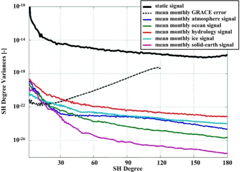
Figure 13.Mean of monthly signal in terms of spherical harmonic degree variances for different mass variation fields compared to mean monthly error from GRACE time variable gravity field es-timates.

is taken into account by dS in the equation above. Loading Love numbers are applied in order to take into account the loading of the mass on the Earth’s crust and the integration is performed by summation over all surface elements. In order to avoid leakage effects, it is important to apply global data sets. For this reason, the atmospheric mass field always rep-resents the basic quantity, because it is the only global field available. Then step-by-step additional sources are added and the final time series represents the simulated global time variable gravity field. The following data combinations were performed:

– Atmosphere only

– Atmosphere & Ocean

– Atmosphere & Ocean & Hydrology

– Atmosphere & Ocean & Hydrology & Ice

– Atmosphere & Ocean & Hydrology & Ice

& Solid-Earth

By this strategy, investigations regarding the gravitational ef-fect of individual mass sources can be performed as well. For example, by subtracting one series from the other one can identify the impact of each individual mass source or of any combination. In the next sub-section a few results are presented. It should be recalled, that the resulting time vari-able gravity field is based on ECMWF reanalysis forcing for the years 1995 to 1999 and on ECMWF operational analysis forcing for the years 2000 to 2006 (see Sect. 2). All mass fields are steady in time and do not exhibit sudden changes, except for the co-seismic signal from the Sumatra earthquake on 26 December 2004 (see Sect. 6).

7.3 Results

In this section, a few examples resulting from this study are shown. Here we only use the resulting spherical harmonic series of the time variable gravity potential in order to char-acterize them.

One way to identify the signal strength of the simulated signal is to compare it with the results for the time vari-able gravity field signal as determined from the GRACE mis-sion. Sensitivity on a global scale can be analyzed by signal and error degree variances (Heiskanen and Moritz, 1967). They show the mean signal or error per degree of a gravity field spherical harmonic series. When comparing the signal degree variances of the simulated fields with the error de-gree variances of the gravity field time series as observed by GRACE (in this case the ITG-GRACE2010S time series is used, see Mayer-G¨urr et al., 2010) one can identify, if a mis-sion is sensitive to the specific time variable gravity signal or not (see Fig. 13).

Figure 13 tells us up to what resolution (in terms of spheri-cal harmonic degree) the time variable signal from individual sources is sensitive for a mission like GRACE. As this rep-resentation is a global average one should regard it as a pes-simistic estimate, which means that for regions with strong mass variability sensitivity could be even higher. We can identify that hydrology exhibits the strongest signal, while for all other sources the signal has a significantly reduced power. With GRACE, one can estimate monthly changes in the continental water at least up to degree 40 (corresponding to 500 km spatial resolution), while for other sources the er-ror line crosses the time variable signal at about degree 20 (corresponding to 1000 km spatial resolution). When inter-preting these results one should not forget that there is still some room to improve the GRACE error curve in future, which would mean higher sensitivity with respect to the in-dividual signals. As this study was designed in preparation for defining future gravity field missions, it is expected that with new gravity field sensors in orbit (laser interferometer) one could reduce the error curve of GRACE by a factor be-tween 20 and 50, which will strongly improve the sensitivity of future missions in terms of spatial resolution. In order to identify the signal versus error for the individual time vari-able gravity field sources for other than monthly periods, the mean variability was computed for 6 hourly, daily, weekly and semi-annual time intervals (see Fig. 14).

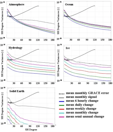
Figure 14. Mean of time variable gravity signals for different time periods in terms of spherical harmonic degree variances compared to mean monthly error from GRACE time variable gravity field estimates. Atmosphere (top left), Ocean (top right), Hydrology (mid left), Ice (mid right), Solid Earth (bottom left).

from space, one needs monthly, or for specific areas with strong signals, weekly observations. Solid Earth processes play a slightly different role, because except for co-seismic events these are very slow processes without seasonal vari-ability. Sudden co-seismic events like earthquakes could have a significant local mass change signal, which is, because of the global mean operator applied for the computation of degree variances, not clearly observable in such representa-tions. In order to have a closer look to the spatial distribu-tion of mass changes, a few monthly maps were computed from the time variable gravity field spherical harmonics (see Fig. 15).

Figure 15.Monthly geoid height maps computed from the spherical harmonic series referenced to the yearly mean for the full time variable gravity signal (atmosphere, oceam hydrology, ice, solid Earth) for two months in 2004 (top row) compared to results obtained from the GRACE mission (bottom row).

with those observed from GRACE (bottom row), for areas with large signal amplitudes good correlations can be iden-tified (global correlation up to 50 %). Due to the design of the GRACE observing system (polar orbit with one dimen-sional observations mostly in North-South direction) we have a non-isotropic error behaviour, which becomes visible by the North-South stripes in the GRACE solutions. Applying specific a-posteriori filter techniques (cf. Kusche, 2007) one could reduce these artefacts significantly with the drawback that some signal is reduced as well. As there is a wide range of filters available, for the correlation analysis shown here the originally observed monthly fields were used. This ensures that the signals’ amplitudes from the geophysical models are comparable to the results from the GRACE data analysis.

From the kind of comparisons shown in the figures above, one can observe that the simulated time variable gravity field as computed from the coupled geophysical models, to a large extent, contains realistic signal amplitudes and frequencies making it is well suited for use in simulating future gravity field missions.

8 Conclusions

In this paper, we have detailed the development of a self-consistent model that realistically describes the motion of mass between the fluid reservoirs of the Earth system. Our model captures mass redistributions between the atmosphere, hydrosphere, oceans, cryosphere and solid Earth and com-bines them into 6-hourly Stokes Coefficients up to degree and order 180 for the period between 1995–2006. The data have been used to test various mission scenarios, e.g. satellite or-bit parameters, allowing us to choose scenarios that optimize

the observability and separability of specific mass transport features. In addition, using a known data set such as this as input, has allowed us to determine the effects of different types of satellite error contributions on the gravity solutions.

Data access

All gravity potential spherical harmonic series including a detailed data format description are available at: http://dx. doi.org/10.1594/PANGAEA.763431 or alternatively at http:

//www.iapg.bv.tum.de/ESA-Mass-Transport.

Acknowledgements. The European Space Agency has provided support for the research that led to this paper in the framework of the study Monitoring and Modelling Individual Sources of Mass Distribution and Transport in the Earth System by Means of Satellites, ESA Contract 20403.

Edited by: G. M. R. Manzella

References

Allen, R. G., Pereira, L. S., Raes, D., and Smith, M.: Crop evapo-transpiration, FAO Irrigation and drainage paper 56, FAO, Rome, 1998.

Andersson, E., Bauer, P., Beljaars, A., Chevallier, F., Holm, E., Janiskova, M., Kallberg, P., Kelly, G., Lopez, P., McNally, A., Moreau, E., Simmons, A. J., Thepaut, J.-N., and Tompkins, A. M.: Assimilation and modelling of the atmospheric hydrological cycle in the ECMWF forecasting system, B. Am. Meteorol. Soc., 86, 387–401, 2005.

J. Hydrometeorol., 10, 953–968, doi:10.1175/2009JHM10341, 2009.

Bougamont, M., Bamber, J. L., and Greuell, W.: A surface mass balance model for the Greenland ice sheet, J. Geophys. Res.-Earth, 110, F04018, doi:10.1029/2005JF000348, 2005. Dobslaw, H.: Modellierung der allgemeinen ozeanischen Dynamik

zur Korrektur und Interpretation von Satellitendaten, Sci. Tech. Rep., STR 07/10, GeoForschungsZentrum Potsdam, 113 pp., 2007.

Dobslaw, H. and Thomas, M.: Atmospheric induced oceanic tides from ECMWF forecasts, Geophys. Res. Lett., 32, L10615, doi:10.1029/2005GL022990, 2005.

Dobslaw, H. and Thomas, M.: Impact of river run-offon global ocean mass redistribution, Geophys. J. Int., 168, 527–532, 2007a.

Dobslaw, H. and Thomas, M.: Simulation and observation of global ocean mass anomalies, J. Geophys. Res., 112, C05040, doi:10.1029/2006JC004035, 2007b.

Drijfhout, S., Heinze, C., Latif, M., and Maier-Reimer, E.: Mean circulation and internal variability in an ocean primitive equation model, J. Phys. Oceanogr., 26, 559–580, 1996.

Dziewonski, M. and Anderson, D. L.: Preliminary reference Earth model. Phys. Earth Planet. In., 25, 297–356, 1981.

Einarsson, I., Hoechner, A., Wang, R., and Kusche, J.: Gravity changes due to the Sumatra-Andaman and Nias earthquakes as detected by the GRACE satellites: a reexamination, Geophys. J. Int., 183, 733–747, doi:10.1111/j.1365-246X.2010.04756.x, 2010.

Farrell, W. E.: Deformation of the Earth by surface loads, Rev. Geo-phys., 10, 761–797, doi:10.1029/RG010i003p00761, 1972. Flechtner, F.: AOD product description document, GRACE 327–

750, rev. 3.1, GeoForschungsZentrum Potsdam, 40 pp., 2007. FAO – Food and Agriculture Organization of the United Nations,

http://www.fao.org/nr/land/soils/digital-soil-map-of-the-world/ en/, last access: 5 October 2011.

Greatbatch, R. J.: A note on the representation of steric sea level in models that conserve volume rather than mass, J. Geophys. Res., 99, 12767–12771, 1994.

Han, S.-C., Shum, C. K., Bevis, M., Ji, C., and Kuo, C.-Y.: Crustal dilatation observed by GRACE after the 2004 Sumatra-Andaman earthquake, Science, 313, 658–662, 2006.

Heiskanen, W. and Moritz, H.: Physical Geodesy, W. H. Freeman & Co Ltd., 1967.

Hellerman, S. and Rosenstein, M.: Normal monthly wind stress over the world ocean with error estimates, J. Phys. Oceanogr., 13, 1093–1104, 1983.

Hibler III, W. D.: A dynamic thermodynamic sea ice model, J. Phys. Oceanogr., 9, 815–846, 1979.

Kusche, J.: Approximate decorrelation and non-isotropic smooth-ing of time-variable GRACE-type gravity field models, J. Geodesy, 81, 733–749, doi:10.1007/s00190-007-0143-3, 2007. Levitus, S.: Climatological atlas of the world ocean, NOAA

Profes-sional Paper, 13, US Department of Commerce, 173 pp., 1982. Mayer-G¨urr, T., Kurtenbach, E., and Eicker, A.: http://www.igg.

uni-bonn.de/apmg/index.php?id=itg-grace2010, last access: 19 October 2011, 2010.

Peltier, W. R.: Global Glacial Isostasy and the Surface of the Ice-Age Earth: The ICE-5G (VM2) Model and GRACE, Ann. Rev. Earth Planet. Sci., 32, 111–149, 2004.

Rignot, E. and Kanagaratnam, P.: Changes in the Velocity Structure of the Greenland Ice Sheet, Science, 311, 986–990, 2006. Rignot, E., Bamber, J. L., van den Broeke, M. R., Davis, C., Li, Y.,

van de Berg, W. J., and van Meijgaard, E.: Recent Antarctic ice mass loss from radar interferometry and regional climate mod-elling, Nat. Geosci., 1, 106–110, doi:10.1038/ngeo102, 2008. Riva, R. E. M., Gunter, B. C., Urban, T. J., Vermeersen, L. L. A.,

Lindenbergh, R. C., Helsen, M. M., Bamber, J. L., van de Wal, R. S. W., van den Broeke, M. R., and Schutz, B. E.: Glacial Isostatic Adjustment over Antarctica from combined ICESat and GRACE satellite data, Earth Planet. Sc. Lett., 288, 516–523, 2009. Sabadini, R. and Vermeersen, L. L. A.: Influence of lithospheric and

mantle layering on global post-seismic deformation, Geophys. Res. Lett., 24, 2075–2078, doi:10.1029/97GL01979, 1997. Sabadini, R. and Vermeersen, L. L. A.: Global Dynamics of the

Earth: Applications of Normal Mode Relaxation Theory to Solid-Earth Geophysics, Vol. 20, Modern Approaches in Geo-physics Series, 344 pp., Kluwer Academic Publishers, ISBN 1-4020-1267-5 (Hardbound), ISBN 1-4020-1268-3 (Paperback), ISBN 1-4020-2135-6 (eBook), 2004.

Schotman, H. H. A. and Vermeersen, L. L. A.: Sensitivity of glacial isostatic adjustment models with shallow low-viscosity earth lay-ers to the ice-load history in relation to the performance of GOCE and GRACE, Earth Planet. Sc. Lett., 236, 828–244, 2005. Simons, M. and Hager, B. H.: Localization of the gravity field and

the signature of glacial rebound, Nature, 390, 500–504, 1997. Tamisiea, M. E., Mitrovica, J. X., and Davis, J. L.: GRACE Gravity

Data Constrain Ancient Ice Geometries and Continental Dynam-ics over Laurentia, Science, 316, 881–883, 2007.

Tapley, B. D., Bettadpur, S., Ries, J. C., Thompson, P. F., and Watkins, M. M.: GRACE Measurements of Mass Variability in the Earth System, Science, 305, 503–506, 2004.

Thomas, M.: Ocean induced variations of Earth’s rotation – Results from a simultaneous model of global circulation and tides, Ph.D. thesis, 129 pp., Univ. of Hamburg, 2002.

Thomas, M., S¨undermann, J., and Maier-Reimer, E.: Considera-tion of ocean tides in an OGCM and impacts on subseasonal to decadal polar motion, Geophys. Res. Lett., 28, 2457–2460, 2001. Troccoli, A. and Kållberg, P.: Precipitation correction in the

ERA-40 reanalysis, ERA-ERA-40 Project Report Series, 13, 2004. Van Beek, L. P. H. and Bierkens, M. F. P.: The Global

Hydrologi-cal Model PCR-GLOBWB: Conceptualization, Parameterization and Verification, Report Department of Physical Geography, Fac-ulty of Earth Sciences Utrecht University, Netherlands, available at: http://vanbeek.geo.uu.nl/suppinfo/vanbeekbierkens2009.pdf, 2009.

Van de Berg, W. J., van den Broeke, M. R., van Meijgaard, E., and Reijmer, C. H.: Reassessment of the Antarctic sur-face mass balance using calibrated output of a regional at-mospheric climate model, J. Geophys. Res., 111, D11104, doi:10.1029/2005JD006495, 2006.

Van den Broeke, M., Bamber, J., Ettema, J., Rignot, E., Schrama, E., van de Berg, W. J., van Meijgaard, E., Velicogna, I., and Wouters, B.: Partitioning Recent Greenland Mass Loss, Science, 326, 984–986, doi:10.1126/science.1178176, 2009.

Velicogna, I.: Increasing rates of ice mass loss from the Green-land and Antarctic ice sheets revealed by GRACE, Geophys. Res. Lett., 36, L19503, doi:10.1029/2009gl040222, 2009.

Satellite Gravity Field Missions in the Post-Goce era, in: Future Satellite Gravimetry and Earth Dynamics, edited by: Flury, J. and Rummel, R., Springer Dordrecht, 2005.

Vermeersen, L. L. A. and Schotman, H. H. A.: High-harmonic geoid signatures related to glacial isostatic adjustment and their detectability by GOCE, J. Geodynamics, 46, 174–181, 2008. Visser, P. N. A. M., Sneeuw, N., Reubelt, T., Losch, M., and van

Dam, T.: Space-borne gravimetric satellite constellations and ocean tides: aliasing effects, Geophys. J. Int., 181, 789–805, doi:10.1111/j.1365-246X.2010.04557.x, 2010.

Wahr, J. M. and Davis, J. L.: Geodetic constraints on glacial iso-static adjustment, in: Ice Sheets, Sea Level and the Dynamic Earth, edited by: Mitrovica, J. X. and Vermeersen, L. L. A., Geo-dynamics Series, 29, American Geophysical Union, Washington, 3–32, 2002.

Walter, C.: Simulation hydrologischer Massenvariationen und deren Einfluss auf die Erdrotation, Diss., Technische Universit¨at Dresden, 196 pp., 2007.

Wolff, J. O., Maier-Reimer, E., and Legutke, S.: The Hamburg Ocean Primitive Equation Model HOPE, Tech. Rep., 13, DKRZ, Hamburg, 103 pp., 1996.