Compressed sensing MRI via fast linearized preconditioned alternating direction method of multipliers

Compressed sensing MRI via fast

linearized preconditioned alternating direction

method of multipliers

Shanshan Chen

_{, Hongwei Du}

_{, Linna Wu}

_{, Jiaquan Jin}

_{and Bensheng Qiu}

Background

Magnetic resonance imaging (MRI), which is non-invasive, provides non-electromag-netic radiation, higher soft-tissue contrast, and spatial resolution, has been applied in diagnostic medicine for many years. However, due to the limitations of the hardware scanning system and the traditional Nyquist sampling theory, MRI scanners take a con-siderable length of time to acquire k-space data. Patient motion (e.g. a beating heart and

Abstract

Background: The challenge of reconstructing a sparse medical magnetic resonance image based on compressed sensing from undersampled k-space data has been investigated within recent years. As total variation (TV) performs well in preserving edge, one type of approach considers TV-regularization as a sparse structure to solve a convex optimization problem. Nevertheless, this convex optimization problem is both nonlinear and nonsmooth, and thus difficult to handle, especially for a large-scale problem. Therefore, it is essential to develop efficient algorithms to solve a very broad class of TV-regularized problems.

Methods: In this paper, we propose an efficient algorithm referred to as the fast linearized preconditioned alternating direction method of multipliers (FLPADMM), to solve an augmented TV-regularized model that adds a quadratic term to enforce image smoothness. Because of the separable structure of this model, FLPADMM decomposes the convex problem into two subproblems. Each subproblem can be alternatively minimized by augmented Lagrangian function. Furthermore, a linearized strategy and multistep weighted scheme can be easily combined for more effective image recovery. Results: The method of the present study showed improved accuracy and efficiency, in comparison to other methods. Furthermore, the experiments conducted on in vivo data showed that our algorithm achieved a higher signal-to-noise ratio (SNR), lower relative error (Rel.Err), and better structural similarity (SSIM) index in comparison to other state-of-the-art algorithms.

Conclusions: Extensive experiments demonstrate that the proposed algorithm exhib-its superior performance in accuracy and efficiency than conventional compressed sensing MRI algorithms.

Keywords: Compressed sensing MRI, Image reconstruction, Total variation, Alternating direction method of multipliers

Open Access

© The Author(s) 2017. This article is distributed under the terms of the Creative Commons Attribution 4.0 International License (http://creativecommons.org/licenses/by/4.0/), which permits unrestricted use, distribution, and reproduction in any medium, provided you give appropriate credit to the original author(s) and the source, provide a link to the Creative Commons license, and indicate if changes were made. The Creative Commons Public Domain Dedication waiver ( http://creativecommons.org/publicdo-main/zero/1.0/) applies to the data made available in this article, unless otherwise stated.

RESEARCH

respiratory movement) during lengthy scans can cause motion and streaking artifacts on the reconstructed image. This degrades image quality, which could lead to misdiagnosis. Thus, accelerating the sampling speed and reducing or eliminating artifacts have always been the aims of many studies.

With the rapid development of the novel compressed sensing (CS) theory [1, 2], com-pressed sensing MRI (CS-MRI) has attracted much attention, as it can reduce imaging time considerably. Compressed sensing theory claims that by using random projection, a small number of data points can be directly sampled at a sampling frequency that is far below the Nyquist frequency. In CS-MRI, the imaging time can be significantly reduced by reconstructing an image of good quality from highly undersampled k-space data. Specifically, if the signal or image is sparse in a certain domain, we can obtain perfect reconstruction with sufficient measurements. MR images are generally sparse in some transform domain, such as the wavelet domain. Consequently, the CS technique can be easily combined with MRI. The original signals or images can be recovered by using the nonlinear reconstruction algorithm under the restricted isometry property (RIP) [3, 4]. Nevertheless, owing to the limitations of MR physics, MRI cannot achieve two-dimen-tional random sampling.

In 2007, Lustig et  al. [5] proposed the SparseMRI algorithm, which selects wavelet transform as a sparse basis, and uses variable density random sampling and the conju-gate gradient descent method for image recovery. This was the first application of CS to MRI. However, due to a high time complexity, the SparseMRI is too slow to be put into practical use. Since then, a variety of nonlinear algorithms have been proposed for CS-MRI reconstruction. The alternatingdirectionmethodofmultipliers (ADMM) algorithm has been studied extensively [6–8], and has been widely used in optimization problems that arise in machine learning, image processing, etc. Recently, the fast alternating direc-tion method of multipliers (FADMM) [9] has incorporated a predictor-corrector accel-eration scheme into the simple ADMM, when a strongly convex condition is satisfied. This algorithm cannot guarantee a global convergence when weakly convex problems are encountered. Another fast method, referred to as the accelerated alternating direc-tion method of multipliers (ALPADMM) [10], was proposed to deal with a class of affine equality constrained composite optimization problems. Although ALPADMM is capable of handling saddle point problems, its convergence rate largely depends on the Lipschitz constant of the smooth component.

similarity (SSIM) index. The main contributions of the work are twofold as follows: (i) the proposed linearized preconditioned alternating direction method of multipliers (FLPADMM) that is inspired by the smooth technique [9], linearized strategy [10, 11], and the accelerated method [10] is designed to solve the augmented TV-regularized model; and (ii) this algorithm only linearizes the closed convex function and does not require the application of multistep weighting to each variable.

The paper is organized as follows: In "Related work", the CS-MRI reconstruction algo-rithms are reviewed. "Methods" briefly describes the basics of CS problem formulation and the proposed FLPADMM method to reconstruct MR images. The experimental results of the proposed approach and comparison with other algorithms are illustrated in "Results". Corresponding discussions are given in "Discussion" and conclusions are provided in "Conclusions".

Related work

In this section, we briefly review the conventional CS-MRI reconstructed algorithms. Many nonlinear algorithms, e.g., the iterative shrinkage/thresholding method (IST) [12], two-step IST (TwIST) scheme [13], fast IST algorithm (FISTA) [14], split augmented Lagrangian shrinkage algorithm (SALSA) [6], wavelet tree sparsity MRI (WaTMRI) [15], total variation augmented Lagrangian alternating direction method (TVAL3) [16], total variation based compressed magnetic resonance imaging (TVCMRI) [17], recon-struction from partial Fourier data (RecPF) [18], and fast composite splitting algorithm (FCSA) [19], have been proposed to improve reconstruction speed and accuracy. IST is an operator-splitting algorithm that can be applied to an optimization problem with a simpler regularization term. The global acceleration of IST may be very slow especially when the stepsize is quite small or the optimization problem is extremely ill-condi-tioned. TwIST, which is a variant of IST, utilizes two or more previous iterates to update the current values, and does not depend on the previous iterate alone. TwIST gains higher speed than IST on reconstruction problem; however, the global convergence rate of TwIST has not been thoroughly studied. FISTA is another accelerated variant of IST that also takes advantage of two previous iterates. Unlike TwIST, FISTA can achieve global convergence with a splitting scheme.

considerably ill-conditioned. Therefore, it is necessary to develop algorithms that are both accurate and efficient to solve large-scale problems.

Methods

Problem formulation

Generally, the classical TV-regularized model for CS-MRI reconstruction problems can be written as:

where x∈Rn is the image to be reconstructed, b∈Rm denotes the undersam-pled k-space data from the MR scanner, and A∈Rm×n_{(m<n) is the measurement}

matrix. The expression δ >0 represents the noise level in the measurement data and (∇x)_i,j=(xi+1,j−xi,j,xi,j+1−xi,j), where ∇ is the discrete gradient operator and |∇x| denotes the TV regularization of x. A variant of (1) is the following TV-regularization problem:

where τ >0 is a positive regularization parameter to balance between the two objec-tives. To enforce image smoothness, we add a quadratic term γ

2�∇x�22 in the objective function to give the new TV-regularized model:

where γ is a smoothing parameter. The augmented term |∇x| +γ₂�∇x�2₂ can yield accu-rate solutions by using a proper value of γ. In addition, the dual problem is continuously differentiable and facilitates effective use of gradient information. To split the variable x, an auxiliary variable z is introduced by ∇x−z=0, and the unconstrained optimization problem (3) is transformed into:

The augmented Lagrangian function for problem (4) is given by:

where ∈Rm is the Lagrangian multiplier, µ is a positive penalty parameter, and

�_,∇x−z� denotes the inner product of the vectors and ∇x−z. The classical ADMM minimizes the convex optimization problem (5) with respect to x and z, using the non-linear block–Gauss–Seidel technique. After minimizing x and z alternatively, can be updated by:

The non-linear block–Gauss–Seidel iteration of ADMM can be written as:

(1) min

x TV(x)|∇x| s.t. �Ax−b�2≤δ,

(2) min

x 1

2�Ax−b� 2

2+τ|∇x|,

(3) min

x 1

2�Ax−b� 2

2+τ|∇x| + γ 2�∇x�

2 2,

(4) min

x 1

2�Ax−b�

2

2+τ|z| +

γ 2�z�

2

2, s.t. ∇x−z=0.

(5)

L(x,z,)= 1

2�Ax−b� 2

2+τ|z| + γ 2�z�

2

2− �,∇x−z� + µ

2�∇x−z� 2 2,

(6)

Suppose z_k and _k are given, then _xk+1 can be obtained by:

When xk+1 and k remain fixed, zk+1 can be minimized by:

The ADMM algorithm above, used to solve (4), is expressed in Algorithm 1.

Algorithm 1ADMM

1: Chooseµ >0,γ >0,τ >0, set k = 1 andλ1= 0 2: repeat

3: xk+1= arg min x

1

2 Ax−b 22−< λk,∇x−zk>+µ2 x−zk 22 4: zk+1= arg min

z τ|z|+ γ

2 z 22−< λk,∇xk+1−z >+µ₂ xk+1−z 2₂ 5: λk+1=λk−µ(∇xk+1−zk+1)

6: k←k+ 1

7: untilstopping criterion is satisfied.

The ADMM has been previously studied and analyzed [7, 8, 20]. Generally, if subprob-lems in (7) are not in closed-form, many solutions could exist within those subprobsubprob-lems. Moreover, when the objective functions are poor or difficult to handle at high precision, the conventional ADMM algorithms might also perform poorly in image reconstruction.

Proposed algorithm

Based on the above analysis, firstly, the minimization of (8) is given by:

Hence, (10) is transformed into:

Because the measurement matrix A is neither the identity matrix, nor is it typically fully dense, it is impossible to derive the exact solution with respect to the x vectors [21]. In addition, the computational cost to handle (11) is extremely heavy. In order to reduce the computational burden and get closed-form solutions, some variants could be con-sidered. The linearization of the quadratic term 1

2�Ax−b�22 is used to update xk+1 as follows: (7)     

x_k+1 ←arg min

x

L_(x,zk,k),

z_k+1 ←arg min_z L(xk+1,z,k),

_k+1 ←_k−µ(∇xk+1−zk+1).

(8)

xk+1=arg min_x 1

2�Ax−b� 2

2− �k,∇x−zk� +

µ

2�∇x−zk� 2 2.

(9) zk+1=arg min_z τ|z| +

γ 2�z�

2

2− �k,∇xk+1−z� + µ

2�∇xk+1−z� 2 2.

(10)

xk+1=arg min_x 1

2�Ax−b� 2

2− �k,∇x−zk� +

µ

2�∇x−zk� 2 2,

=arg min

x

1

2�Ax−b� 2 2+

µ 2�∇x−

zk+

_k

µ

�2₂.

(11)

(ATA+µ∇T∇)x_k+1=ATb+ ∇T(µzk+k).

(12) 1

2�Ax−b� 2 2≈

1

2�Axk−b� 2

2+ �Grad(xk),x−xk� + η

where Grad(x_k)=AT(Ax_k −b) is the gradient of 1₂�Ax−b�2₂ at the current point x_k, and η is a positive proximal parameter. Then, the x subproblem in (10) can be iterated by:

Considering the quadratic term µ

2�∇x−zk�22 can also be linearized, we also linearize

µ

2�∇x−zk�22 at xk. This variant is a fast linearized preconditioned ADMM(FLPADMM) algorithm that generates the iterates x_k+1 by:

The negative divergence operator −div can be used to solve (14) as follows:

Secondly, for a given x_k+1 and k, zk+1 is computed by solving:

Hence, the solution to (16) obeys:

where soft(·,T) is the soft thresholding function that is defined as:

Finally, the Lagrangian multiplier is updated by _k+1=_k−µ(∇xk+1−zk+1).

(13) x_k+1=arg min

x �Grad(xk),x−xk� + η

2�x−xk�

2 2

− �_k,∇x−zk� + µ

2�∇x−zk�

2 2.

(14) x_k+1=arg min

x

L_(x,zk,k),

=arg min x

1

2�Ax−b�

2

2− �k,∇x−zk� +

µ

2�∇x−zk�

2 2,

=arg min

x �Grad(xk),x−xk� +

η

2�x−xk�

2

2− �k,∇x�

+ �µ(∇xk−zk),∇x�,

=arg min

x �Grad(xk),x−xk� +

η

2�x−xk�

2 2

+ �µ(∇xk−zk)−k,∇x�.

(15) x_k+1=xk−

1

η(−div(µ(∇xk−zk)−k)+Grad(xk)).

(16) zk+1=arg min

z

L_(xk+1,z,k),

=arg min z τ|z| +

γ

2�z�

2

2− �k,∇xk+1−z� + µ

2�∇xk+1−z�

2 2,

=arg min z τ|z| +

γ

2�z�

2 2+

µ

2�z−

∇xk+1−

_k

µ

�2₂,

=arg min z τ|z| +

γ +µ

2 �z−

µ γ +µ

∇xk+1−

_k

µ

�2₂,

=arg min z

τ γ +µ|z| +

1 2�z−

µ γ +µ

∇x_k+1−

_k

µ

�2₂.

(17) zk+1=soft

µ γ +µ

∇xk+1−

_k

µ

, τ γ +µ

,

(18) soft(v,T)=

 



v+T, v<−T, 0, |v| ≤ |T|,

The FLPADMM algorithm utilizes the gradient descent method and one soft thresh-olding operator to update variables at each iteration. In addition, this method is a variant of the classical ADMM algorithm framework. The proposed FLPADMM algorithm is presented in Algorithm 2.

Algorithm 2FLPADMM

1: Chooseµ1>0,γ1>0,η1>0,τ1>0, Set k = 1,xw

1 =x1andλ1= 0 2: repeat

3: αk=_k1 4: xm

k = (1−αk)xwk+αkxk

5: xk+1=xk−_η1_k(−div(µk(∇xk−zk)−λk) +Grad(xmk)) 6: xw

k+1= (1−αk)xwk+αkxk+1 7: zk+1=sof t( µk

γk+µk(∇xk+1−

λk

µk),

τk

γk+µk)

8: λk+1=λk−µk(∇xk+1−zk+1) 9: k←k+ 1

10: untilstopping criterion is satisfied.

The stopping criterion in all of the algorithms above is the relative change of x between two successive iterations, which is small enough, i.e.:

where tol is usually a range chosen from 10−5 to 10−3. In the FLPADMM algorithm, α_k represents a weighted parameter and Grad(xm_k) is the gradient of 1₂�Ax−b�22 at the point xm_k. Furthermore, xm_k is the first weighted value that is used to update x_k+1.

It should be noted that the appropriate parameter α_k can improve the rate of conver-gence that has been proven in a previous study [10]. Moreover, the superscript m stands for “middle,” and w stands for “weight.” Before the gradient descent method in line 5 is applied, x is updated by the weighted sums of all previous iterates. Furthermore, after the gradient method is applied, x is updated again by the same weighting technique, that is, x is weighted twice at each iteration. Specifically, when the weighted parameter α_k is set to 1, the x subproblem is simply the current point xk+1. At this point, FLPADMM becomes another variant of the ADMM algorithm [10]. The accelerated strategy of FLPADMM incorporates a multistep acceleration scheme with middle point xm and weighted point xw, which was first applied in a previous study [10] and derived from the accelerated gradient method [22, 23]. Moreover, the optimal rate of convergence of FLPADMM is O

1 k2 + 1_k

.

Results

Experimental setup

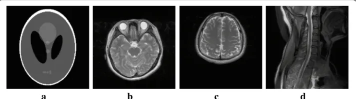
A series of numerical experiments were conducted to compare the performance of the proposed FLPADMM with two state-of-the-art algorithms, namely FADMM [9] and ALPADMM [10], for MR image reconstruction from undersampled k-space data. The four typical MR datasets (Shepp–Logan phantom, human brain1 MR data, human brain2 MR data, and human spine MR data) were used to evaluate our algorithm. All test images had the same matrix size of 256 × 256, as shown in Fig. 1a–d. The first Shepp– Logan phantom was a piecewise smooth image with pixel intensities ranging from 0 to 1. The complex k-space data of the human brain1 was acquired from a 3T GE MR750 (19) �xk+1−xk�2

scanner using the FRFSE sequence (TR = 6000 ms, TE = 101 ms). The human brain2 data was also obtained from the 3T GE MR750 system (TR/TE = 2500/96.9 ms, field of view = 280 × 280 mm, slice thickness = 5 mm). The human spine MR data was fully sampled k-space data acquired on a 3T GE MR750 system with a FRFSE sequence (TR/ TE = 2500/110 ms, field of view = 240 × 240 mm, slice thickness = 5 mm). To achieve fair comparisons, codes of all compared algorithms were downloaded from the authors’ websites. All experiments were executed, using Windows 10 and MATLAB 2015b (64-bit), on a desktop computer with a 3.2GHz Intel core i5-4460 CPU and 8GB of RAM.

Each experiment was repeated 10 times, and the average image metric results of 10 experiments were recorded. For most of the MR images, the k-space signals with a large magnitude were generally localized in the central region. Since a non-Cartesian sam-pling matrix is incoherent, the results on the Cartesian masks were far less favorable than those on the non-Cartesian mask. Therefore, two non-Cartesian masks were cho-sen as the sampling masks. One was a pseudo-Gaussian mask, displayed in Fig. 2a, that was implemented by following the sampling strategy of collecting more low-frequency signals in the central part of the k-space, and less high-frequency signals in the periph-eral part of the k-space. The other mask presented in Fig. 2b, was a pseudo-radial mask that was applied by following the rule of RecPF [18]. The sampling ratio was defined as the number of sampled points divided by the total size of the original image.

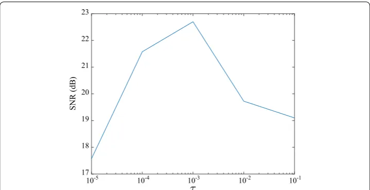
In the present study, we compared our algorithm with two state-of-the-art algorithms under similar conditions. To explore the influence of the regularization parameter τ, we

a b c d

Fig. 1 MR images. (a) Shepp–Logan phantom (b) human brain1 image (c) human brain2 image (d) human spine image

a b

used human brain1 data as an example, to analyze the changes of image quality when τ was changed. In Fig. 3, the SNR attained the maximum value when τ was 10−3. Thus, we chose this optimum value to achieve favorable reconstruction. Similar searches were adopted for the other datasets. For all tests, we also found that when γ =2τ, our algo-rithm maintained the most favorable reconstruction performance. Furthermore, the default maximum of all three methods was set to 300.

To quantitatively evaluate the result of the proposed algorithm, three objective metrics were adopted to measure the quality of the recovered images. The first was SNR, defined as:

where x is the original image, ∧x is the reconstructed image, and M and N represent the number of rows and columns, respectively, in the input image. The quality of the recon-structed image is directly proportional to the value of SNR. The second metric was the Rel.Err, defined as:

A smaller value meant that the reconstructed image had little error and more favorable reconstruction in comparison to the original image.

The last metric was the SSIM index that was used to measure the similarity between two images, in terms of structure, brightness, and contrast, among other aspects, and defined as:

(20) SNR=10 log₁₀

M

i=0 N

j=0x(i,j)2

M

i=0 N

j=0(x(i,j)−

∧

x(i,j))2 ,

(21) Rel.Err= �x−

∧

x�₂

�x�₂ ×100%.

(22)

SSIM(p,q)= (2µpµq+c1)(2θpq+c2) (µ2_p+µ2_p+c1)(θp2+θq2+c2)

,

10-5 ₁₀-4 ₁₀-3 ₁₀-2 ₁₀-1

17 18 19 20 21 22 23

SNR (dB)

where µp and θp are the mean and variance, respectively, of the original image; µq and θq are the mean and variance, respectively, of the reconstructed image, θpq is the covariance of these two images; and c1 and c2 are fixed constants that prevent unstable phenom-ena when the denominator is close to zero. When the value of SSIM was increased, the image showed greater similarity to the original.

Experimental results

In this section, we first compare our proposed FLPADMM algorithm with FADMM [9] and ALPADMM [10] algorithms on the Shepp–Logan phantom, with Gaussian white noise of a standard deviation of 0.01. The proposed FLPADMM was applied to the Shepp–Logan phantom under pseudo-Gaussian mask with 20% k-space data under-sampled. Figure 4a shows the original Shepp–Logan phantom, and Fig. 4b–d presents the reconstructed images recovered by the FADMM, ALPADMM, and FLPADMM algorithms, respectively. Compared with the original Shepp–Logan phantom image, FADMM yielded noticeable artifacts and failed to suppress background noise. The image recovered by ALPADMM contained fewer artifacts and was evidently more favorable than that recovered by FADMM. As the Shepp–Logan phantom is extremely piecewise smooth and sparse, ALPADMM also provides good reconstruction. As shown in Fig. 4c, d, visible artifacts are not easily observed when both ALPADMM and FLPADMM are used. However, for experiments on in vivo data as we will show, FLPADMM would per-form much more accurately and stably than ALPADMM.

For enhanced visualization, Fig. 4e–g depicts the difference between the reconstructed image and the original image of the Shepp–Logan phantom under a pseudo-Gauss-ian mask at a sampling ratio of 20% using FADMM, ALPADMM, and the proposed FLPADMM reconstruction. It was evident that the reconstruction with FLPADMM had

a b c d

e f g

the smallest error. The proposed FLPADMM exhibited superior performance in sup-pressing noise without significant artifacts, and yielded the best reconstruction.

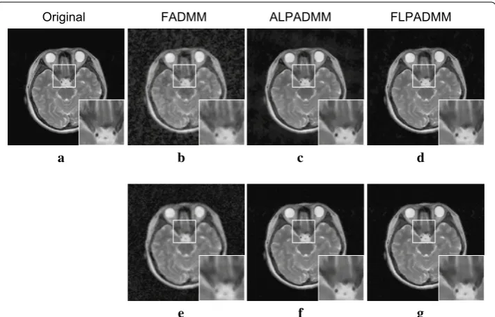
All experiments on in vivo data were corrupted with Gaussian white noise with zero mean and a standard deviation of 0.01. Experimental results of these in  vivo human brain data are displayed in Figs. 5 and 6 at a sampling ratio of 25%. Figure 5a presents the original human brain1 image. The reconstructed images illustrated in Fig. 5b–d, were obtained by FADMM, ALPADMM, and our proposed FLPADMM, under a pseudo-Gaussian sampling scheme. Figure 5e–g was produced by FADMM, ALPADMM, and FLPADMM, respectively, under a pseudo-radial sampling pattern. The SNR of the human brain1 image under the pseudo-Gaussian mask using FLPADMM was 25.0685 dB, whereas those recovered by FADMM and ALPADMM were 20.9921 and 22.3231 dB, respectively. We can clearly see that the FLPADMM reconstruction suppressed back-ground noise. The recovery result in Fig. 6 is similar to that in Fig. 5.

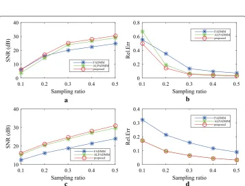
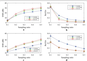
Figure 7 gives the comparison results of human brain1 data among the state-of-the-art MR image reconstruction algorithms, using different sampling masks, when the sam-pling ratios were 0.1, 0.2, 0.3, 0.4, and 0.5, respectively. As seen in Fig. 7a, b, the proposed FLPADMM achieved high image quality with high SNR and low Rel.Err. When the sam-pling ratio was 0.1, the three methods performed relatively poorly. That is because when sampling ratio is too low, the sampled data is insufficient to obtain a faithful image. It is notable that as the sampling ratio increased for all algorithms under consideration, the SNR was also increased, whereas Rel.Err was gradually reduced. That is, the recon-structions of higher quality could have been obtained by taking more measurements. In addition, when the sampling ratio was increased, the FLPADMM algorithm exhibited superior performance in recovering the sampling image. Specifically, a sampling ratio of 30% was sufficient to reconstruct the human brain1 image effectively.

Original

a

FADMM

b

ALPADMM

c

FLPADMM

d

e f g

Figure 8 shows the comparison results of human brain2 data, where (a) and (c) present the SNR of the human brain2 image with different ratios, and (b) and (d) describe the Rel.Err of the human brain2 image at different ratios. The results are similar to those

Original

a

FADMM

b

ALPADMM

c

FLPADMM

d

e f g

Fig. 6 Reconstructed images and zoomed-in regions among the state-of-the-art MR image reconstruction algorithms using a pseudo-Gaussian mask (first row) and pseudo-radial mask (second row) with 25% sampling. a Original human brain1 image, b, e FADMM, c, f ALPADMM, d, g FLPADMM

0.1 0.2 0.3 0.4 0.5

Sampling ratio 0

10 20 30 40

SNR (dB)

a

FADMM ALPADMM proposed

0.1 0.2 0.3 0.4 0.5

Sampling ratio 0

0.2 0.4 0.6 0.8

Rel.Er

r

b

FADMM ALPADMM proposed

0.1 0.2 0.3 0.4 0.5

Sampling ratio 10

20 30 40

SNR (dB

)

c

FADMM ALPADMM proposed

0.1 0.2 0.3 0.4 0.5

Sampling ratio 0

0.1 0.2 0.3 0.4

Rel.Er

r

d

FADMM ALPADMM proposed

of the human brain1 image. The SNR of FLPADMM was slightly larger than that of ALPADMM when a pseudo-radial mask was applied. The Rel.Err of ALPADMM was very close to that of FLPADMM (see Figs. 7d, 8d), indicating that both ALPADMM and our proposed FLPADMM show similar recovery performance under the pseudo-radial mask.

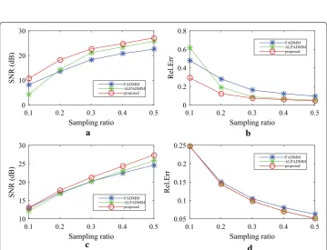
The reconstructed results in Fig. 9 were consistent with those of Fig. 5. Compared to FADMM and ALPADMM, our proposed FLPADMM reconstructed better images without visual artifacts. For example, when the sampling ratio was 25% under pseudo-radial sampling, FADMM had significant artifacts and ALPADMM had slight artifacts. However, images reconstructed by FLPADMM were the closest to the original image of the human spine. These results further validate the superiority of FLPADMM in com-parison to other algorithms and are consistent with the results of the two human brain experiments. It is clear that regardless of the sampling scheme, FLPADMM achieved the highest SNR and lowest Rel.Err. From Fig. 10, we can see that all reconstruction results showed steady improvement as the sampling ratio increased. Moreover, FLPADMM showed superior performance in comparison to other algorithms. As the tissue structure of the human spine MR data was extremely complex, the quality of the reconstructed image was not as good as that of the human brain tests.

For further comparison, the results of quantitative image metrics, SSIM and CPU time (s), are listed in Tables 1 and 2 to demonstrate structural similarity and running time of FADMM, ALPADMM, and FLPADMM algorithms for all MR images at vari-ous sampling ratios. As seen in Table 2, the running time of FLPADMM was faster than that of ALPADMM, but slower than that of FADMM by approximately 1 s. Since the

0.1 0.2 0.3 0.4 0.5

Sampling ratio 0

10 20 30 40

SNR (dB)

a

FADMM ALPADMM proposed

0.1 0.2 0.3 0.4 0.5

Sampling ratio 0

0.2 0.4 0.6 0.8

Rel.Er

r

b

FADMM ALPADMM proposed

0.1 0.2 0.3 0.4 0.5

Sampling ratio 10

20 30 40

SNR (dB

)

c

FADMM ALPADMM proposed

0.1 0.2 0.3 0.4 0.5

Sampling ratio 0

0.1 0.2 0.3 0.4

Rel.Er

r

d

FADMM ALPADMM proposed

convergence of FADMM was also close to O( 1

k2) when strict conditions were satisfied, the running time of all three methods were very similar. According to the value of the SSIM, the proposed FLPADMM achieved higher quality images than the other techniques.

Original

a

FADMM

b

ALPADMM

c

FLPADMM

d

e f g

Fig. 9 Reconstructed images and zoomed-in regions among the state-of-the-art MR image reconstruction algorithms using a pseudo-Gaussian mask (first row) and pseudo-radial mask (second row) with 25% sampling. a Original human brain1 image, b, e FADMM, c, f ALPADMM, d, g FLPADMM

0.1 0.2 0.3 0.4 0.5

Sampling ratio 0

10 20 30

SNR (dB)

a

FADMM ALPADMM proposed

0.1 0.2 0.3 0.4 0.5

Sampling ratio 0

0.2 0.4 0.6 0.8

Rel.Er

r

b

FADMM ALPADMM proposed

0.1 0.2 0.3 0.4 0.5

Sampling ratio 10

15 20 25 30

SNR (dB

)

c

FADMM ALPADMM proposed

0.1 0.2 0.3 0.4 0.5

Sampling ratio 0.05

0.1 0.15 0.2 0.25

Rel.Er

r

d

FADMM ALPADMM proposed

Table 1 Additional reconstruction results on different MR images with a pseudo-Gaussian mask under different sample ratios

The CPU time and SSIM comparison among FADMM, ALPADMM, and the proposed FLPADMM Test image Metric Algorithm Sampling ratio

0.1 0.2 0.3 0.4 0.5

Human brain1 SSIM FADMM 0.3493 0.4497 0.7052 0.9707 0.9842 ALPADMM 0.1470 0.5126 0.9748 0.9836 0.9904 FLPADMM 0.3981 0.5241 0.9788 0.9869 0.9918 CPU time (s) FADMM 2.9609 3.0238 3.0955 3.1921 3.6528 ALPADMM 4.2605 4.3840 4.4864 4.6043 4.7250 FLPADMM 4.0840 4.3312 4.4342 4.5427 4.5791 Human brain2 SSIM FADMM 0.2786 0.3702 0.7391 0.9828 0.9914 ALPADMM 0.1631 0.4244 0.9877 0.9922 0.9955 FLPADMM 0.3325 0.4215 0.9911 0.9944 0.9961 CPU time (s) FADMM 3.0527 3.2095 3.2354 3.2802 3.2332 ALPADMM 4.3250 4.4526 4.7770 4.5932 4.6251 FLPADMM 4.2333 4.4974 4.5447 4.4557 4.6193 Human spine SSIM FADMM 0.2077 0.3270 0.4755 0.5528 0.6200 ALPADMM 0.4396 0.7779 0.9425 0.9672 0.9807 FLPADMM 0.6235 0.7869 0.9731 0.9830 0.9889 CPU time (s) FADMM 2.9718 3.0915 3.1162 3.1401 3.1521 ALPADMM 4.3979 4.4857 4.6409 4.5899 4.6300 FLPADMM 4.3400 4.4285 4.4914 4.5481 4.6091

Table 2 Additional reconstruction results on  different MR images with  a pseudo-radial mask under different sample ratios

The CPU time and SSIM comparison among FADMM, ALPADMM, and the proposed FLPADMM Test image Metric Algorithm Sampling ratio

0.1 0.2 0.3 0.4 0.5

Discussion

We proposed a novel algorithm for CS-MRI reconstruction, referred to as FLPADMM. Except for the TV-regularization term in the classical MR model, we added a quadratic term to this classical model to make the image smoother. Using augmented Lagrangian function, FLPADMM effectively divides the original convex problem into two subprob-lems, both of which can be easily dealt with. To further enhance image reconstruction, a strategy that incorporated a multistep weighted scheme was adopted in FLPADMM. Several parameters need to be tuned in our proposed algorithm. In general, the require-ment on stepsize η obeys η > µATA. When the regularization parameter τ is 10−3 (see Fig. 3) and γ =2τ, our proposed algorithm yields the best result. The other parameters can be manually set for different test data under a fixed sampling scheme. When differ-ent sampling schemes (i.e., pseudo-Gaussian mask and pseudo-radial mask) are applied, our proposed FLPADMM can also produce very impressive results. Experiments vali-date that the performance of this proposed method is superior to those of FADMM and ALPADMM. It particularly shows the best performance in suppressing background noise, even at a low sampling ratio.

Some algorithms that combine parallel MRI and CS have been proposed to acceler-ate MRI reconstruction [24–26]. Our method can also be applied to parallel MRI with minor revisions.

Conclusions

The consideration of TV-regularization for CS-MRI has been studied within recent years, largely because MR images can be recovered from its partial Fourier samples, and TV shows better performance in preserving image edges. In this paper, we first briefly reviewed nonlinear algorithms for CS-MRI, and then introduced an augmented TV-regularized model with an additional quadratic term to enforce image smoothness. An efficient, inexact, but unique algorithm has been proposed to handle this novel TV-regularized model. The proposed algorithm, referred to as FLPADMM, belongs to the classical ADMM framework that decomposes the objective function into two subprob-lems by adding new variables and constraints. FLPADMM minimizes the TV-regular-ized objective function by an augmented Lagrangian minimization function technique. Furthermore, this method effectively adopts a multistep weighted scheme to improve the accuracy of reconstruction. Moreover, FLPADMM could also solve both constrained and unconstrained convex optimization problems. Numerous experiments demonstrate the superiority of the proposed FLPADMM method in comparison to the previous FADMM and ALPADMM algorithms. Our future work would combine this algorithm with parallel MRI to further accelerate the imaging time.

Abbreviations

Authors’ contributions

CSS conceived the study and participated in its design, implemented the algorithm, performed the acquisition of MR images, carried out the experiments, analyzed the data and drafted the manuscript. DHW participated in the design of the study, performed critical revision of the manuscript for important intellectual content and obtained funding. WLN also performed the acquisition of MR images and helped to draft the manuscript. JJQ drew some of the figures and supervised the study. QBS expressed opinions on the overall framework of the manuscript. All authors read and approved the final manuscript.

Author details

1 _{Center for Biomedical Engineering, Department of Electronic Science and Technology, University of Science and} Tech-nology of China, Heifei 230027, China. 2 _{Department of Radiology, University of Washington School of Medicine, Seattle,} WA 98108, USA. 3 _{Anhui Computer Application Institute of Traditional Chinese Medicine, Hefei 230038, China.}

Acknowledgements

The authors would like to thank the Centers for Biomedical Engineering, University of Science and Technology of China for providing the 3T GE MR750 scanner. The authors are also grateful to the anonymous reviewers for their valuable com-ments and suggestions.

Competing interests

The authors declare that they have no competing interests.

Availability of data and materials

All datasets related to the current study are available from the corresponding author on reasonable request.

Consent for publication

In this study, all of the experiments were agreed upon by the volunteers and Centers for Biomedical Engineering, Univer-sity of Science and Technology of China, Heifei, China. In addition, all MR datasets would be published.

Ethics approval and consent to participate

The ethical approval was given by the Medical Ethics Committee of the University of Science and Technology of China, Heifei, China.

Funding

This work was supported by the National Natural Science Foundation of China under Grant No .81527802.

Publisher’s Note

Springer Nature remains neutral with regard to jurisdictional claims in published maps and institutional affiliations.

Received: 16 December 2016 Accepted: 22 April 2017

References

1. Donoho DL. Compressed sensing. IEEE Trans Inf Theory. 2006;52(4):1289–306.

2. Lustig M, Donoho DL, Santos JM, Pauly JM. Compressed sensing MRI. IEEE Signal Process Mag. 2008;25(2):72–82. 3. Candès EJ, Wakin MB. An introduction to compressive sampling. IEEE Signal Process Mag. 2008;25(2):21–30. 4. Candès EJ, Romberg J, Tao T. Robust uncertainty principles: Exact signal reconstruction from highly incomplete

frequency information. IEEE Trans Inf Theory. 2006;52(2):489–509.

5. Lustig M, Donoho D, Pauly JM. Sparse MRI: The application of compressed sensing for rapid MR imaging. Magn Reson Med. 2007;58(6):1182–95.

6. Afonso MV, Bioucas-Dias JM, Figueiredo MA. Fast image recovery using variable splitting and constrained optimiza-tion. IEEE Trans Image Process. 2010;19(9):2345–56.

7. Eckstein J, Bertsekas DP. On the Douglas-Rachford splitting method and the proximal point algorithm for maximal monotone operators. Math Program. 1992;55(1–3):293–318.

8. Glowinski R, Le Tallec P. Augmented Lagrangian and operator-splitting methods in nonlinear mechanics, vol. 9; 1989. 9. Goldstein T, O’Donoghue B, Setzer S, Baraniuk R. Fast alternating direction optimization methods. SIAM J Imaging

Sci. 2014;7(3):1588–623.

10. Ouyang Y, Chen Y, Lan G, Pasiliao E Jr. An accelerated linearized alternating direction method of multipliers. SIAM J Imaging Sci. 2015;8(1):644–81.

11. Yang Z-Z, Yang Z. Fast linearized alternating direction method of multipliers for the augmented\ ell _1-regularized problem. Signal Image Video Process. 2015;9(7):1601–12.

12. Daubechies I, Defrise M, De Mol C. An iterative thresholding algorithm for linear inverse problems with a sparsity constraint. Commun Pure Appl Math. 2004;57(11):1413–57.

13. Bioucas-Dias JM, Figueiredo MA. A new twist: two-step iterative shrinkage/thresholding algorithms for image resto-ration. IEEE Trans Image Process. 2007;16(12):2992–3004.

14. Beck A, Teboulle M. A fast iterative shrinkage-thresholding algorithm for linear inverse problems. SIAM J Imaging Sci. 2009;2(1):183–202.

• We accept pre-submission inquiries

• Our selector tool helps you to find the most relevant journal • We provide round the clock customer support

• Convenient online submission • Thorough peer review

• Inclusion in PubMed and all major indexing services • Maximum visibility for your research

Submit your manuscript at www.biomedcentral.com/submit

Submit your next manuscript to BioMed Central

and we will help you at every step:

16. Li C. An efficient algorithm for total variation regularization with applications to the single pixel camera and com-pressive sensing. PhD thesis, Citeseer; 2009.

17. Ma S, Yin W, Zhang Y, Chakraborty A. An efficient algorithm for compressed MR imaging using total variation and wavelets. In: Computer vision and pattern recognition, 2008. IEEE conference on CVPR; 2008. p 1–8.

18. Yang J, Zhang Y, Yin W. A fast alternating direction method for tvl1-l2 signal reconstruction from partial fourier data. IEEE J Sel Top Signal Process. 2010;4(2):288–97.

19. Huang J, Zhang S, Metaxas D. Efficient MR image reconstruction for compressed MR imaging. Med Image Anal. 2011;15(5):670–9.

20. Gabay D, Mercier B. A dual algorithm for the solution of nonlinear variational problems via finite element approxi-mation. Comput Math Appl. 1976;2(1):17–40.

21. Monteiro RD, Svaiter BF. Iteration-complexity of block-decomposition algorithms and the alternating direction method of multipliers. SIAM J Optim. 2013;23(1):475–507.

22. Nesterov Y. A method for unconstrained convex minimization problem with the rate of convergence o (1/k2). Doklady an SSSR. 1983;269:543–7.

23. Nesterov Y. Introductory lectures on convex optimization: a basic course vol. 87; 2013.

24. Chang Y, King KF, Liang D, Wang Y, Ying L. A kernel approach to compressed sensing parallel MRI. In: 2012 9th IEEE international symposium on biomedical imaging (ISBI). IEEE; 2012. p. 78–81.

25. Liu B, Zou YM, Ying L. Sparsesense: application of compressed sensing in parallel MRI. In: 2008 international confer-ence on information technology and applications in biomedicine. IEEE; 2008. p. 127–30.