Comparative performance of an elitist teaching-learning-based optimization algorithm for solving unconstrained optimization problems Pages 29-50 Download PDF

(1)

International Journal of Industrial Engineering Computations 4 (2013) 29–50

Contents lists available at GrowingScience

International Journal of Industrial Engineering Computations

homepage: www.GrowingScience.com/ijiec

Comparative performance of an elitist teaching-learning-based optimization algorithm for solving unconstrained optimization problems

R. Venkata Rao*and Vivek Patel

Department of Mechanical Engineering, S.V. National Institute of Technology, Ichchanath, Surat, Gujarat – 395 007, India A R T I C L E I N F O A B S T R A C T

Article history:

Received 11 July 2012 Received in revised format 14 August 2012

Accepted August 31 2012 Available online 1 September 2012

Teaching-Learning-based optimization (TLBO) is a recently proposed population based algorithm, which simulates the teaching-learning process of the class room. This algorithm requires only the common control parameters and does not require any algorithm-specific control parameters. In this paper, the effect of elitism on the performance of the TLBO algorithm is investigated while solving unconstrained benchmark problems. The effects of common control parameters such as the population size and the number of generations on the performance of the algorithm are also investigated. The proposed algorithm is tested on 76 unconstrained benchmark functions with different characteristics and the performance of the algorithm is compared with that of other well known optimization algorithms. A statistical test is also performed to investigate the results obtained using different algorithms. The results have proved the effectiveness of the proposed elitist TLBO algorithm.

Keywords:

Teaching-learning-based optimization; Elitism Population size Number of generations Unconstrained optimization problems

1. Introduction

Some of the recognized evolutionary algorithms are, Genetic Algorithms (GA), Differential Evolution (DE), Evolution Strategy (ES), Evolution Programming (EP), Artificial Immune Algorithm (AIA), Bacteria Foraging Optimization (BFO), etc. Among all, GA is a widely used algorithm for various applications. GA works on the principle of the Darwinian theory of the survival of the fittest and the theory of evolution of the living beings (Holland 1975). DE is similar to GA with specialized crossover and selection method (Storn & Price 1997, Price et al. 2005). ES is based on the hypothesis that during the biological evolution the laws of heredity have been developed for fastest phylogenetic adaptation (Runarsson & Yao, 2000). ES imitates, in contrast to the GA, the effects of genetic procedures on the phenotype. EP also simulates the phenomenon of natural evolution at phenotype level (Fogel et al.

(2)

Frog Leaping (SFL) algorithm which works on the principle of communication among the frogs (Eusuff & Lansey, 2003); Artificial Bee Colony (ABC) algorithm which works on the principle of foraging behavior of a honey bee (Karaboga, 2005; Basturk & Karaboga 2006; Karboga & Basturk, 2007-2008; Karaboga & Akay 2009).

There are some other algorithms which work on the principles of different natural phenomena. Some of them are: Harmony Search (HS) algorithm which works on the principle of music improvisation in a music player (Geem et al. 2001); Gravitational Search Algorithm (GSA) which works on the principle of gravitational force acting between the bodies (Rashedi et al. 2009); Biogeography-Based Optimization (BBO) which works on the principle of immigration and emigration of the species from one place to the other (Simon, 2008); Grenade Explosion Method (GEM) which works on the principle of explosion of grenade (Ahrari & Atai, 2010); and League championship algorithm which mimics the sporting competition in a sport league (Kashan, 2011).

All the evolutionary and swarm intelligence based algorithms are probabilistic algorithms and required common controlling parameters like population size and number of generations. Beside the common control parameters, different algorithm requires its own algorithm specific control parameters. For example GA uses mutation rate and crossover rate. Similarly PSO uses inertia weight, social and cognitive parameters. The proper tuning of the algorithm specific parameters is very crucial factor which affect the performance of the above mentioned algorithms. The improper tuning of algorithm-specific parameters either increases the computational effort or yields the local optimal solution. Considering this fact, recently Rao et al. (2011, 2012a, 2012b) and Rao and Patel (2012a) introduced the Teaching-Learning-Based Optimization (TLBO) algorithm which does not require any algorithm-specific parameters. TLBO requires only common controlling parameters like population size and number of generations for its working. Thus, TLBO can be said as an algorithm-specific parameter-less algorithm.

The concept of elitism is utilized in most of the evolutionary and swarm intelligence algorithms where during every generation the worst solutions are replaced by the elite solutions. The number of worst solutions replaced by the elite solutions is depended on the size of elite. Rao and Patel (2012a) described the elitism concept while solving the constrained benchmark problems. The same methodology is extended in the present work and the performance of TLBO algorithm is investigated considering a number of unconstrained benchmark problems. The details of TLBO algorithm along with its computer program are available in Rao and Patel (2012a) and hence those details are not repeated in this paper.

2. Elitist TLBO algorithm

(3)

algorithm is 500000. The next section deals with the experimentation of the elitist TLBO algorithm on various unconstrained benchmark functions.

3. Experiments on unconstrained benchmark functions

The considered unconstrained benchmark functions have different characteristics like unimodality/multimodality, separability/non-separability and regularity/non-regularity. In this section three different experiments are conducted to identify the performance of TLBO and compare the performance of TLBO algorithm with other evolutionary and swarm intelligence based algorithms. A common platform is provided by maintaining the identical function evolution for different algorithms considered for the comparison. Thus, the consistency in the comparison is maintained while comparing the performance of TLBO with other optimization algorithms. However, in general, the algorithm which requires less number of function evaluations to get the same best solution can be considered as better as compared to the other algorithms. If an algorithm gives global optimum solution within certain number of function evaluations, then consideration of more number of function evaluations will go on giving the same best result. Rao et al. (2011, 2012a) showed that TLBO requires less number of function evaluations as compared to the other optimization algorithms. However, in this paper, to maintain the consistency in comparison, the number of function evaluations of 500000, 100000 and 5000 is maintained for experiments 1, 2 and 3 respectively for all optimization algorithms including TLBO algorithm.

3.1. Experiment 1

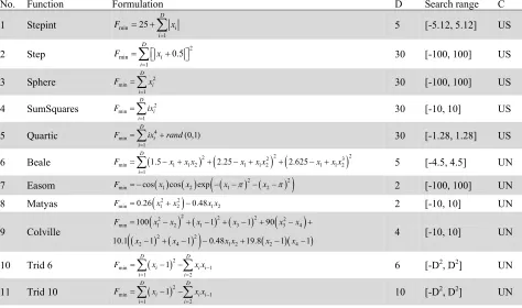
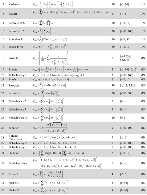
In the first experiment, the TLBO algorithm is implemented on 50 unconstrained benchmark functions taken from the previous work of Karaboga and Akay (2009). The details of the benchmark functions considered in this experiment are shown in Table 1.

Table 1

Benchmark functions considered in experiment 1, D: Dimension, C: Characteristic, U: Unimodal, M: Multimodal, S: Separable, N: Non-separable

No. Function Formulation D Search range C

1 Stepint min

1 25

D i i

F x

=

= +

∑

5 [-5.12, 5.12] US

2 Step min 2

1 0.5

D i i

F x

=

⎡ ⎤

=

∑

_⎣ + _⎦ 30 [-100, 100] US

3 Sphere 2

min 1

D i i

F x

=

∑

₃₀ _{[-100, 100]} _US

4 SumSquares 2

min 1

D i i

F ix

=

∑

30 [-10, 10] US

5 Quartic 4

min 1

(0,1) D

i i

F ix rand

=

∑

+ ₃₀ _{[-1.28, 1.28]} _US

6 Beale ( )2

(

2

) (

2 3

)

2

min 1 1 2 1 1 2 1 1 2

1

1.5 2.25 2.625

D

i

F x x x x x x x x x

=

∑

− + + − + + − + _{5 [-4.5,}_{4.5] UN}

7 Easom Fmin= −cos( ) ( )x1 cos x2 exp

(

−(x1−π) (2− x2−π)2

)

2 [-100, 100] UN

8 Matyas

(

2 2

)

min 0.26 1 2 0.481 2

F = x +x − x x 2 [-10, 10] UN

9 Colville

(

)

( ) ( )

(

)

( ) ( )

(

)

( )( )

2 2 2

2 2

min 1 2 1 3 3 4

2 2

2 4 1 2 2 4

100 1 1 90

10.1 1 1 0.48 19.8 1 1

F x x x x x x

x x x x x x

= − + − + − + − +

− + − − + − − 4 [-10, 10] UN

10 Trid 6 min ( )2 1

1 2

1

D D

i i i

i i

F x x x−

= =

=

∑

− −

∑

_{6 [-D}2_{, D}2_{] UN}

11 Trid 10 min ( )2 1

1 2

1

D D

i i i

i i

F x x x−

= =

(4)

Table 2

Benchmark functions considered in experiment 1, D: Dimension, C: Characteristic, U: Unimodal, M: Multimodal, S: Separable, N: Non-separable (Cont.)

12 Zakharov

2 4

2 min

1 1 1

0.5 0.5

D D D

i i i

F x ix ix

= = =

⎛ ⎞ ⎛ ⎞

= +⎜ ⎟ +⎜ ⎟

⎝ ⎠ ⎝ ⎠

∑

10 [-5, 10] UN

13 Powell ( ) ( ) ( ) ( )

/ 4

2 2 4 4

min 4 3 4 2 4 1 4 4 2 4 1 4 3 4

1

10 5 10 10

D

i i i i i i i i

i

F x − x − x − x x − x − x − x

=

∑

+ + − + + + −

24 [-4, 5] UN

14 Schwefel 2.22 min

1 1

D D

i i

F x x

= =

=

∑ ∏

+ _{30 [-10,}_10] _UN

15 Schwefel 1.2

2 2 min 1 1 D i j i j F x = = ⎛ ⎞ = ⎜_⎜ ⎟_⎟ ⎝ ⎠

∑ ∑

30 [-100, 100] UN

16 Rosenbrock 2 2 2

min 1

1

[100( ) (1 ) ]

D

i i i

i

F x x₊ x

=

∑

− + − 30 [-30, 30] UN

17 Dixon-Price ( )2

(

2

)

2

min 1 1

2

1 2

D

i i

i

F x i x x−

=

= − +

∑

− ₃₀ _{[-10, 10]} _UN

18 Foxholes

(

)

1

25

min 2 ₆

1 1 1 1 500 _j i ij i F

j x a

− = = ⎡ ⎤ ⎢ ⎥ ⎢ ⎥ =_⎢ + _⎥ + − ⎢ ⎥ ⎣ ⎦

∑

2 [-65.536,

65.536] MS

19 Branin

2 2

min 2 2 1 1 1

5.1 5 ₆ _{10 1} 1 _cos ₁₀

8 4

F x x _πx _π x

π

⎛ ⎞ ⎛ ⎞

=_⎜ − + − _⎟ + _⎜ − _⎟ +

⎝ ⎠ ⎝ ⎠ 2 [-5, 10] [0, 15] MS

20 Bohachevsky 1 2 2 ( ) ( )

min 1 2 2 0.3cos 3 1 0.4cos 4 2 0.7

F =x + x − πx − πx + 2 [-100, 100] MS

21 Booth ( ) (2 )2

min 1 2 2 7 21 2 5

F = x − x − + x +x − 2 [-10, 10] MS

22 Rastrigin 2

min 1

10cos(2 ) 10

D

i i

i

F x πx

=

⎡ ⎤

=

∑

_⎣ − + _⎦ 30 [-5.12, 5.12] MS

23 Schwefel min

(

( )

)

1

sin

D

i i

i

F x x

=

= −

∑

30 [-500, 500] MS

24 Michalewicz 2

20 2 min 1 1 sin sin D i i ix

F x _π

=

⎛ ⎛ ⎞⎞

= − ⎜ ⎜ ⎟⎟

⎝ ⎠

∑

2 [0, π] MS

25 Michalewicz 5

F x _π

=

⎛ ⎛ ⎞⎞

= − ⎜ ⎜ ⎟⎟

⎝ ⎠

∑

5 [0, π] MS

26 Michalewicz 10

F x _π

=

⎛ ⎛ ⎞⎞

= − ⎜ ⎜ ⎟⎟

⎝ ⎠

∑

10 [0, π] MS

27 Schaffer

(

)

(

)

(

)

2 2 2 1 2

min ₂ ₂ 2

1 2 sin 0.5 0.5 1 0.001 x x F x x + − = +

+ + 2 [-100, 100] MN

28 6 Hump _CamelBack 2 4 6 2 4

min 1 1 1 1 2 2 2

1

4 2.1 4 4

3

F = x − x + x +x x − x + x 2 [-5, 5] MN

29 Bohachevsky 2 2 2 ( )( )

min 1 2 2 0.3cos 3 1 4 2 0.3

F =x + x − πx πx + 2 [-100, 100] MN

30 Bohachevsky 3 2 2 ( )

min 1 2 2 0.3cos 3 1 4 2 0.3

F =x + x − πx + πx + 2 [-100, 100] MN

31 Shubert

(

( )

)

(

( )

)

5 5

min 1 2

1 1

cos 1 cos 1

i i

F i i x i i i x i

= =

⎛ ⎞⎛ ⎞

=⎜ + + ⎟⎜ + + ⎟

⎝

∑

⎠⎝

∑

⎠ 2 [-10, 10] MN

32 GoldStein-Price ( )

(

)

( )

(

)

2 2 2

min 1 2 1 1 2 1 2 2

2 2 2

1 2 1 1 2 1 2 2

1 1 19 14 3 14 6 3

30 2 3 18 32 12 48 36 27

F x x x x x x x x

x x x x x x x x

⎡ ⎤

= +_⎣ + + − + − + + _⎦

⎡ ₊ ₋ ₋ ₊ ₊ ₋ ₊ ⎤

⎣ ⎦

2 [-2, 2] MN

33 Kowalik

(

)

2 2 11

1 2

min 2

1 3 4

i i

i

i i i

x b b x

F a

b b x x = ⎛ ₊ ⎞ ⎜ ⎟ = − ⎜ + + ⎟ ⎝ ⎠

∑

4 [-5, 5] MN

34 Shekel 5 ( )( )

5 1

min 1

T

i i i

i

F x a x a c

−

=

⎡ ⎤

= −

∑

_⎣ − − + _⎦ _{4 [0,}_10] _MN

35 Shekel 7 min 7 ( )( ) 1 1

T

i i i

i

F x a x a c

−

=

⎡ ⎤

(5)

Table 2

Benchmark functions considered in experiment 1, D: Dimension, C: Characteristic, U: Unimodal, M: Multimodal, S: Separable, N: Non-separable (Cont.)

36 Shekel 10 ( )( )

10 1

min 1

T

i i i

i

F x a x a c

−

=

⎡ ⎤

= −

∑

_⎣ − − + _⎦ _{4 [0,}_10] _MN

37 Perm

(

)

2 min 1 1 1 k D D k i k i x F i i β = = ⎡ ⎛_⎛ _⎞ ⎞⎤ = ⎢ + ⎜_⎜⎜ ⎟ − ⎟_⎟⎥ ⎝ ⎠ ⎢ ⎝ ⎠⎥ ⎣ ⎦

∑ ∑

4 [-D, D] MN

38 PowerSum 2 min 1 1 D D k i k k i

F x b

= =

⎡⎛ ⎞ ⎤

= ⎢⎜ ⎟− ⎥

⎢⎝ ⎠ ⎥

⎣ ⎦

∑ ∑

4 [0, D] MN

39 Hartman 3

(

)

4 3 ₂

min

1 1

exp

i ij j ij

i j

F c a x p

= =

⎡ ⎤

= − ⎢− − ⎥

⎢ ⎥

⎣ ⎦

∑

3 [0, 1] MN

40 Hartman 6

(

)

4 6 ₂

min

1 1

exp

i ij j ij

i j

F c a x p

= =

⎡ ⎤

= − ⎢− − ⎥

⎢ ⎥

⎣ ⎦

∑

6 [0, 1] MN

41 Griewank 2

min 1 1 1 cos 1 4000 D D i i i i x F x i = = ⎛ ⎞ = − _⎜ _⎟+ ⎝ ⎠

∑ ∏

30 [-600, 600] MN

42 Ackley 2

min

1 1

20exp 0.2 exp cos 2 20

D D

i i

F x x e

D = D = π

⎛ ⎞ _⎛ _⎞

⎜ ⎟

= − _⎜− _⎟− ⎜ ⎟+ +

⎝ ⎠

⎝

∑

⎠

∑

30 [-32, 32] MN

43 Penalized

{

}

1

2 2 2 2

min 1 1

1

10sin ( ) ( 1) 1 10sin ( ) ( 1)

( ) ,

( ,10,100, 4), ( , , , ) 0, ,

( ) ,

1 1 / 4( 1) D

i i D

i

m

i i

D

i i i

i _m

i i

F y y y y

D

k x a x a

u x u x a k m a x a

k x a x a

y x π _π − _π + = = ⎡ ⎤ = ⎢ + − + + − ⎥ ⎣ ⎦

⎧ − >

⎪

+ =⎨ − ≤ ≤

⎪ − − < −

⎩

= + +

∑

30 [-50, 50] MN

44 Penalized 2

{

}

(

)

2 2 2

1 ₁

2

min 1 ₂

1

( 1) 1 sin (3 ) ( 1)

0.1 sin ( )

1 sin (2 )

( ) ,

( ,5,100,4), ( , , , ) 0, ,

( ) ,

D

i i D

i _D

m

i i

D

i i i

i m

i i

x x x

F x

x

k x a x a

u x u x a k m a x a

k x a x a

π π π − ₊ = = ⎡ ₋ ₊ ₊ ₋ ⎤ ⎢ ⎥ = + ⎢ _{+ +} ⎥ ⎣ ⎦

⎧ − >

⎪

+ =⎨ − ≤ ≤

⎪ − − < −

⎩

∑

30 [-50, 50] MN

45 Langerman 2 min

(

)

2

(

)

2

1 1 1

1

exp cos

D D D

i j ij j ij

i j j

F c x a π x a

π = = = ⎛ ⎛ ⎞ ⎛ ⎞⎞ ⎜ ⎟ = − _⎜ ⎜_⎜− − ⎟_⎟ ⎜_⎜ − ⎟_⎟_⎟ ⎝ ⎠ ⎝ ⎠ ⎝ ⎠

∑

2 [0, 10] MN

46 Langerman 5 min

(

)

2

(

)

2

1 1 1

1

exp cos

D D D

i j ij j ij

i j j

F c x a π x a

π = = = ⎛ ⎛ ⎞ ⎛ ⎞⎞ ⎜ ⎟ = − _⎜ ⎜_⎜− − ⎟_⎟ ⎜_⎜ − ⎟_⎟_⎟ ⎝ ⎠ ⎝ ⎠ ⎝ ⎠

∑

5 [0, 10] MN

47 Langerman 10 min

(

)

2

(

)

2

1 1 1

1

exp cos

D D D

i j ij j ij

i j j

F c x a π x a

π = = = ⎛ ⎛ ⎞ ⎛ ⎞⎞ ⎜ ⎟ = − _⎜ ⎜_⎜− − ⎟_⎟ ⎜_⎜ − ⎟_⎟_⎟ ⎝ ⎠ ⎝ ⎠ ⎝ ⎠

∑

10 [0, 10] MN

48 FletcherPowell 2 ( )

(

)

(

2 min

1 1 1

sin cos , sin cos

D D D

i i i ij j ij j i ij j ij

i j j

F A B A a α b α B a x b

= = =

=

∑

− =

∑

+ =

∑

+

2 [-π, π] MN

49 FletcherPowell 5 ( )

(

)

(

2 min

1 1 1

sin cos , sin cos

D D D

i j j

= = =

=

∑

− =

∑

+ =

∑

+

5 [-π, π] MN

50 FletcherPowell ₁₀ ( )

(

)

(

2 min

1 1 1

sin cos , sin cos

D D D

i j j

= = =

=

∑

− =

∑

+ =

∑

+

10 [-π, π] MN

(6)

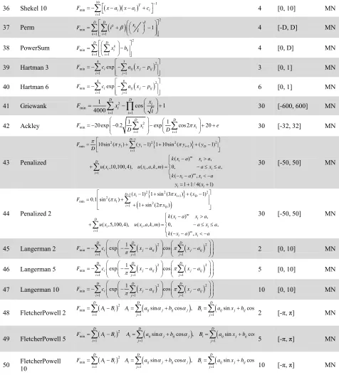
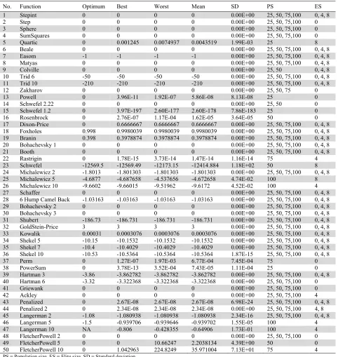
9850, 4850, 3183 and 2350 respectively so that the function evaluations in each strategy is 500000. Similarly, to identify the effect of elite size on the performance of the algorithm, the algorithm is experimented with different elite sizes, viz. 0, 4, and 8. Here elite size 0 indicates no elitism consideration. The results of each benchmark function are presented in Table 2 in the form of best solution, worst solution, average solution and standard deviation obtained in 30 independent runs on each benchmark function along with the corresponding strategy (i.e. population size and elite size).

Table 2

Results Obtained by the TLBO algorithm for 50 bench mark functions over 30 independent runs with 500000 function evaluations

No. Function Optimum Best Worst Mean SD PS ES

1 Stepint 0 0 0 0 0.00E+00 25, 50, 75,100 0, 4, 8

2 Step 0 0 0 0 0.00E+00 25, 50, 75,100 0

3 Sphere 0 0 0 0 0.00E+00 25, 50, 75,100 0

4 SumSquares 0 0 0 0 0.00E+00 25, 50, 75,100 0

5 Quartic 0 0.001245 0.0074937 0.0043519 1.99E-03 25 8

6 Beale 0 0 0 0 0.00E+00 25, 50, 75,100 0, 4, 8

7 Easom -1 -1 -1 -1 0.00E+00 25, 50, 75,100 0, 4, 8

8 Matyas 0 0 0 0 0.00E+00 25, 50, 75,100 0, 4, 8

9 Colville 0 0 0 0 0.00E+00 25, 50 0, 4, 8

10 Trid 6 -50 -50 -50 -50 0.00E+00 25, 50, 75,100 0, 4, 8

11 Trid 10 -210 -210 -210 -210 0.00E+00 25, 50, 75,100 0, 4, 8

12 Zakharov 0 0 0 0 0.00E+00 25, 50, 75 0

13 Powell 0 3.96E-11 1.92E-07 5.86E-08 8.13E-08 25 0

14 Schwefel 2.22 0 0 0 0 0.00E+00 25, 50 0

15 Schwefel 1.2 0 3.97E-197 2.60E-177 2.60E-178 7.86E-183 25 0

16 Rosenbrock 0 2.76E-07 1.17E-04 1.62E-05 3.64E-05 50 0

17 Dixon-Price 0 0.6666667 0.6666667 0.6666667 0.00E+00 25, 50, 75,100 0, 4, 8

18 Foxholes 0.998 0.9980039 0.9980039 0.9980039 0.00E+00 25, 50, 75,100 0, 4, 8

19 Branin 0.398 0.3978874 0.3978874 0.3978874 0.00E+00 25, 50, 75,100 0, 4, 8

20 Bohachevsky 1 0 0 0 0 0.00E+00 25, 50, 75,100 0, 4, 8

21 Booth 0 0 0 0 0.00E+00 25, 50, 75,100 0, 4, 8

22 Rastrigin 0 1.78E-15 3.73E-14 1.47E-14 1.16E-14 75 4

23 Schwefel -12569.5 -12569.49 -12173.15 -12414.884 1.18E+02 50 8

24 Michalewicz 2 -1.8013 -1.801303 -1.801303 -1.801303 0.00E+00 25, 50, 75,100 0, 4, 8

25 Michalewicz 5 -4.6877 -4.687658 -4.537656 -4.672658 4.74E-02 100 8

26 Michalewicz 10 -9.6602 -9.66015 -9.51962 -9.6172 4.52E-02 100 4

27 Schaffer 0 0 0 0 0.00E+00 25, 50, 75,100 0, 4, 8

28 6 Hump Camel Back -1.03163 -1.03163 -1.03163 -1.03163 0.00E+00 25, 50, 75,100 0, 4, 8

29 Bohachevsky 2 0 0 0 0 0.00E+00 25, 50, 75,100 0, 4, 8

30 Bohachevsky 3 0 0 0 0 0.00E+00 25, 50, 75,100 0, 4, 8

31 Shubert -186.73 -186.731 -186.731 -186.731 0.00E+00 25, 50, 75,100 0, 4, 8

32 GoldStein-Price 3 3 3 3 0.00E+00 25, 50, 75,100 0, 4, 8

33 Kowalik 0.00031 0.0003076 0.0003076 0.0003076 0.00E+00 25, 50, 75,100 0, 4, 8

34 Shekel 5 -10.15 -10.1532 -10.1532 -10.1532 0.00E+00 25, 50, 75,100 0, 4, 8

35 Shekel 7 -10.4 -10.4029 -10.4029 -10.4029 0.00E+00 25, 50, 75,100 0, 4, 8

36 Shekel 10 -10.53 -10.5364 -10.5364 -10.5364 1.87E-15 25, 50, 75,100 0, 4, 8

37 Perm 0 1.27E-07 1.97E-03 6.77E-04 7.45E-04 75 0

38 PowerSum 0 3.78E-13 3.52E-04 7.43E-05 1.11E-04 25 0

39 Hartman 3 -3.86 -3.862782 -3.862782 -3.862782 0.00E+00 25, 50, 75,100 0, 4, 8

40 Hartman 6 -3.32 -3.322368 -3.322368 -3.322368 0.00E+00 25, 50, 75,100 0

41 Griewank 0 0 0 0 0.00E+00 25, 50, 75,100 0

42 Ackley 0 0 0 0 0.00E+00 25, 50, 75,100 4

43 Penalized 0 2.67E-08 2.67E-08 2.67E-08 6.98E-24 25, 50, 75,100 0, 4, 8

44 Penalized 2 0 2.34E-08 2.34E-08 2.34E-08 0.00E+00 25, 50, 75,100 4, 8

45 Langerman 2 -1.08 -1.080938 -1.080938 -1.080938 2.34E-16 25, 50, 75,100 0, 4, 8

46 Langerman 5 -1.5 -0.939706 -0.939646 -0.939702 1.55E-05 100 4

47 Langerman 10 NA -0.806 -0.428355 -0.64906 1.73E-01 100 4

48 FletcherPowell 2 0 0 0 0 0.00E+00 25, 50, 75,100 0

49 FletcherPowell 5 0 0 10.66247 2.2038134 4.39E+00 50 0

50 FletcherPowell 10 0 1.042963 224.8249 35.971004 7.13E+01 75 4

PS = Population size, ES = Elite size, SD = Standard deviation

(7)

and 49, strategy with population size of 50 and number of generations of 4850 gave the best results. For functions 22, 37 and 50, strategy with population size of 75 and number of generations of 3183 and for functions 25, 26, 46 and 47 strategy with population size of 100 and number of generations of 2350 produced the best results. For function 12, strategy with population size 25, 50 and 75 while for function 9 and 14, strategy with population size 25 and 50 produced the identical results. For rest of the functions all the strategies produced the same results and hence there is no effect of population size on these functions to achieve their respective global optimum values with same number of function evaluations.

Similarly, it is observed from Table 2 that for functions 2-4, 12-16, 37, 38, 40, 41, 48 and 49, strategy with elite size 0, i.e. no elitism produced best results than the other strategies having different elite sizes. For functions 22, 26, 42, 46, 47 and 50, strategy with elite size of 4 produced the best results. For functions 5, 23, and 25, strategy with elite size of 8 produced the best results. For function 44, strategy with elite size 4 and 8 produced the same results. For rest of the functions all the strategies (i.e. strategy without elitism consideration as well as strategies with different elite sizes consideration) produced the same results.

The performance of TLBO algorithm is compared with the other well known optimization algorithms such as GA, PSO, DE and ABC. The results of GA, PSO, DE and ABC are taken from the previous work of Karaboga and Akay (2009) where the authors had experimented benchmark functions each with 500000 function evaluations with best setting of algorithm specific parameters. Table 3 shows the comparative results of the considered algorithm in the form of mean solution (M), standard deviation (SD) and standard error of mean (SEM). In order to maintain the consistency in the comparison the values bellow 10-12_{are assumed to be 0 as considered in the previous work of Karaboga and Akay}

(2009). It is observed from Table 3 that TLBO algorithm outperforms the GA, PSO, DE and ABC algorithms for Powell, Rosenbrock, Kowalik, Perm, and Power sum functions in every aspect of comparison criteria. For Rastrigin, Hartman 6, and Griewank functions, performance of the TLBO and ABC algorithms are alike and outperforms the GA, PSO and DE algorithms. For Shekel 5, Shekel 7, Shekel 10, Hartman 3, and Ackley functions, performance of the TLBO, DE and ABC algorithms are alike and outperforms the GA and PSO algorithms. For Colville function, performance of PSO and TLBO while for Zakharov function, performance of TLBO, DE and PSO are same and produce better results.

(8)

Table 3

Comparative results of TLBO with other evolutionary algorithms over 30 independent runs

Function

GA PSO DE ABC TLBO Function GA PSO DE ABC TLBO

Stepint

M 0 0 0 0 0

Step

M 1.17E+03 0 0 0 0

SD

0.00E+00 0 0 0 SD0 76.56145 0 0 0 0

SEM 0.00E+00 0 0 0 0 SEM 13.978144 0 0 0 0

Sphere

M 1.11E+03 0 0 0 0

Sum Squares

M 1.48E+02 0 0 0 0

SD

74.214474 0 0 0 SD0 12.409289 0 0 0 0

SEM 13.549647 0 0 0 0 SEM 2.265616 0 0 0 0

Quartic

M 0.1807 0.001156 0.001363 0.030016 0.004351

Beale

M 0 0 0 0 0

SD

0.027116 0.000276 0.000417 0.004866 1.99E-03 SD 0 0 0 0 0

SEM 0.004951 5.04E–05 7.61E–05 0.000888 3.64E-04 SEM 0 0 0 0 0

Easom

M -1 -1 -1 -1 -1

Matyas

M 0 0 0 0 0

SD 0 0 0 0 SD0 0 0 0 0 0

SEM 0 0 0 0 0 SEM 0 0 0 0 0

Colville

M 0.014938 0 0.0409122 0.0929674 0

Trid 6

M -49.9999 -50 -50 -50 -50

SD

0.007364 0.0819790 0.066277 SD0 2.25E–5 0 0 0 0

SEM 0.001344 0 0.014967 0.0121 0 SEM 4.11E–06 0 0 0 0

Trid 10

M -209.476 -210 -210 -210 -210

Zakharov

M 0.013355 0 0 0.0002476 0

SD

0.193417 0 0 0 SD0 0.004532 0 0.0001830 0

SEM 0.035313 0 0 0 0 SEM 0.000827 0 0 3.34E–05 0

Powell

M 9.703771 0.00011 2.17E–07 0.0031344 5.86E-08

Schwefel 2.22

M 11.0214 0 0 0 0

SD

1.547983 0.00016 1.36E–7 0.000503 8.13E-08 SD 1.386856 0 0 0 0

SEM 0.282622 2.92E–05 2.48E–08 9.18E–05 1.48E-08 SEM 0.253204 0 0 0 0

Schwefel 1.2

M 7.40E+03 0 0 0 0

Rosenbrock

M 1.96E+05 15.088617 18.203938 0.0887707 1.62E-05

SD

1.14E+03 0 0 0 SD0 3.85E+04 24.170196 5.036187 0.07739 3.64E-05

SEM 208.1346 0 0 0 0 SEM 7029.1062 4.412854 0.033333 0.014129 6.65E-06

(9)

Table 3

Comparative results of TLBO with other evolutionary algorithms over 30 independent runs (Cont.)

Function PSOGA DE ABC TLBO Function PSOGA DE ABC TLBO

Dixon-Price

M 1.22E+03 0.6666667 0.6666667 0 0.6666667

Foxholes

M 0.998004 0.9980039 0.9980039 0.9980039 0.9980039

SD

2.66E+02 E–8 E–9 0 SD0 0 0 0 0 0

SEM 48.564733 1.82E–09 1.82E–10 0 0 SEM 0 0 0 0 0

Branin

M 0.397887 0.3978874 0.3978874 0.3978874 0.3978874

Bohachevsky 1

M 0 0 0 0 0

SD 0 0 0 0 SD0 0 0 0 0 0

SEM 0 0 0 0 0 SEM 0 0 0 0 0

Booth

M 0 0 0 0 0

Rastrigin

M 52.92259 43.977137 11.716728 0 0

SD 0 0 0 0 SD0 4.56486 11.728676 2.538172 0 0

SEM 0 0 0 0 0 SEM 0.833426 2.141353 0.463405 0 0

Schwefel

M -11593.4 -6909.1359 -10266 -12569.487 -12414.884

Michalewicz 2

M -1.8013 -1.5728692 -1.801303 -1.8013034 -1.801303

SD

93.25424 457.95778 521.84929 0.00E+00 1.18E+02 SD 0.00E+00 0.11986 0 0 0

SEM 17.025816 83.611269 95.28 0.00E+00 2.15E+01 SEM 0.00E+00 0.021883 0 0 0

Michalewicz 5

M -4.64483 -2.4908728 -4.683482 -4.6876582 -4.6726578

Michalewicz 10

M -9.49683 -4.0071803 -9.591151 -9.6601517 -9.6172

SD

0.09785 0.256952 0.012529 0.00E+00 4.74E-02 SD 0.141116 0.502628 0.064205 4.52E-020

SEM 0.017865 0.046913 0 0 8.66E-03 SEM 0.025764 0.091767 0.011722 0 8.24E-03

Schaffer

M 0.004239 0 0 0 0

Six Hump CamelBack

M -1.03163 -1.032 -1.032 -1.032 -1.03163

SD

0.004763 0 0 0 SD0 0 0 0 0 0

SEM 0.00087 0 0 0 0 SEM 0 0 0 0 0

Bohachevsky 2

M 0.06829 0.00 0.00 0.00 0.00

Bohachevsky 3

M 0.00 0.00 0.00 0.00 0.00

SD

0.078216 0.00 0.00 0.00 0.00 SD 0.000.00 0.00 0.00 0.00

SEM 0.01428 0.00 0.00 0.00 0.00 SEM 0.00 0.00 0.00 0.00 0.00

Shubert

M -186.731 -186.73091 -186.7309 -186.73091 -186.7309

GoldStein-Price

M 5.250611 3 3 3 3

SD 0 0 0 0 SD0 5.870093 0 0 0 0

(10)

Table 3

Comparative results of TLBO with other evolutionary algorithms over 30 independent runs (Cont.)

Function PSOGA DE ABC TLBO Function PSOGA DE ABC TLBO

Kowalik

M 0.005615 0.0004906 0.0004266 0.0004266 0.0003076

Shekel 5

M -5.66052 -2.0870079 -10.1532 -10.1532 -10.1532

SD

0.008171 0.000366 0.000273 6.04E–5 SD0 3.866737 1.17846 0 0 0

SEM 0.001492 6.68E–05 4.98E–05 1.10E–05 0 SEM 0.705966 0.215156 0 0 0

Shekel 7

M -5.34409 -1.9898713 -10.40294 -10.402941 -10.4029

Shekel 10

M -3.82984 -1.88 -10.54 -10.54 -10.5364

SD

3.517134 1.420602 0 0 SD0 2.451956 0.432476 0 0 0

SEM 0.642138 0.259365 0 0 0 SEM 0.447664 0.078959 0 0 0

Perm

M 0.302671 0.0360516 0.0240069 0.0411052 0.0006766

PowerSum

M 0.010405 11.390448 0.0001425 0.0029468 0.0000743

SD

0.193254 0.048927 0.046032 0.023056 0.0007452 SD 0.009077 7.3558 0.000145 0.002289 0.0001105

SEM 0.035283 0.008933 0.008404 0.004209 0.000136 SEM 0.001657 1.342979 2.65E–05 0.000418 2.02E-05

Hartman 3

M -3.86278 -3.6333523 -3.862782 -3.8627821 -3.862782

Hartman 6

M -3.29822 -1.8591298 -3.226881 -3.3219952 -3.322368

SD

0.00E+00 0.116937 0 0 SD0 0.05013 0.439958 0.047557 0 0

SEM 0.00E+00 0.02135 0 0 0 SEM 0.009152 0.080325 0.008683 0 0

Griewank

M 10.63346 0.0173912 0.0014792 0 0

Ackley

M 14.67178 0.1646224 0 0 0

SD

1.161455 0.020808 0.002958 0 SD0 0.178141 0.493867 0 0 0

SEM 0.212052 0.003799 0.00054 0 0 SEM 0.032524 0.090167 0 0 0

Penalized

M 13.3772 0.0207338 0 0 2.67E-08

Penalized 2

M 125.0613 0.0076754 0.0021975 0 2.34E-08

SD

1.448726 0.041468 0 0 SD0 12.0012 0.016288 0.004395 0 0

SEM 0.2645 0.007571 0 0 0 SEM 2.19111 0.002974 0.000802 0 0

Langerman 2

M -1.08094 -0.679268 -1.080938 -1.0809384 -1.080938

Langerman 5

M -0.96842 -0.5048579 -1.499999 -0.93815 -0.939702

SD 0.2746210 0 0 SD0 0.287548 0.213626 0.0002080 1.55E-05

SEM 0 0.050139 0 0 0 SEM 0.052499 0.039003 0 3.80E–05 2.83E-06

Langerman 10

M -0.63644 -0.0025656 -1.0528 -0.4460925 -0.64906

Fletcher Powell 2

M 0 0 0 0 0

SD

0.374682 0.003523 0.302257 0.133958 0.1728623 SD 0 0 0 0 0

SEM 0.068407 0.000643 0.055184 0.024457 0.03156 SEM 0 0 0 0 0

Fletcher Powell 5

M 0.004303 1457.8834 5.988783 0.1735495 2.2038134

Fletcher Powell 10

M 29.57348 1364.4556 781.55028 8.2334401 35.971004

SD

0.009469 1269.3624 7.334731 0.068175 4.3863209 SD 16.02108 1325.3797 1048.8135 8.092742 71.284369

(11)

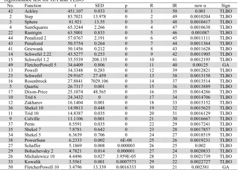
Table 4

Significance test for GA and TLBO

No.

Function SEDt p IRR new Signα

42 Ackley 451.107 0.033 0 1 50 0.001 TLBO

2

Step 83.7021 13.978 0 2 49 TLBO0.0010204

3 Sphere 81.921 13.55 0 3 48 0.0010417 TLBO

4

SumSquares 65.3244 2.266 0 474 0.0010638 TLBO

22 Rastrigin 63.5001 0.833 0 5 46 0.001087 TLBO

44

Penalized 57.07672 2.191 0 456 0.0011111 TLBO

43 Penalized 50.5754 0.264 0 7 44 0.0011364 TLBO

41

Griewank 50.1456 0.212 0 8 43 TLBO0.0011628

14 Schwefel 2.22 43.5277 0.253 0 9 42 0.0011905 TLBO

15

Schwefel 35.55391.2 208.135 100 41 0.0012195 TLBO

49 FletcherPowell 5 34.6409 0.806 0 11 40 0.00125 GA

13

Powell 34.3348 0.283 120 39 0.0012821 TLBO

23 Schwefel 29.9167 27.459 0 13 38 0.0013158 TLBO

16

Rosenbrock 27.8841 7029.106 0 14 37 TLBO0.0013514

5 Quartic 26.7317 0.001 0 15 36 0.0013889 TLBO

17

Dixon-Price 25.1074 48.565 160 35 0.0014286 TLBO

10 Trid 6 24.3432 0 0 17 34 0.0014706 TLBO

12

Zakharov 16.1404 0.001 180 33 0.0015152 TLBO

36 Shekel 10 14.9813 0.448 0 19 32 0.0015625 TLBO

11

Trid 14.838710 0.035 200 31 0.0016129 TLBO

9 Colville 11.1106 0.001 0 21 30 0.0016667 TLBO

37

Perm 8.5591 0.035 220 29 0.0017241 TLBO

35 Shekel 7 7.8781 0.642 0 23 28 0.0017857 TLBO

34

Shekel 6.36395 0.706 240 27 0.0018519 TLBO

38 PowerSum 6.2333 0.002 6E-08 25 26 0.0019231 TLBO

27

Schaffer 5.1869 0.008 0.000003 26 25 0.002 TLBO

29 Bohachevsky 2 4.7821 0.014 0.000001 27 24 0.0020833 TLBO 26

Michalewicz 4.449610 0.027 3.959E-05 28 23 0.0021739 TLBO

33 Kowalik 3.5561 0.001 0.0007573 29 22 0.0022727 TLBO

50

FletcherPowell 3.479610 13.339 0.0016333 30 21 0.002381 GA t: t-value of student t-test, SED: standard error of difference, p: p-value calculated for t-value, R: rank of p-value, IR: Inverse rank of p-value, Sign: Significance

Table 5

Significance test for PSO and TLBO

No.

23 Schwefel 63.7666 86.342 0 1 50 0.001 TLBO

26

Michalewicz 60.888110 0.092 0 2 49 TLBO0.00102

25 Michalewicz 5 45.7345 0.048 0 3 48 0.001042 TLBO

34

Shekel 37.48995 0.215 0 474 0.001064 TLBO

36 Shekel 10 33.3766 0.259 0 5 46 0.001087 TLBO

35

Shekel 32.43727 0.259 0 456 0.001111 TLBO

22 Rastrigin 20.5371 2.141 0 7 44 0.001136 TLBO

40

Hartman 18.21656 0.08 0 438 0.001163 TLBO

47 Langerman 10 16.6788 0.032 0 9 42 0.00119 TLBO

46

Langerman 11.14915 0.039 100 41 0.00122 TLBO

39 Hartman 3 10.7463 0.021 0 11 40 0.00125 TLBO

24

Michalewicz 10.43872 0.022 120 39 0.001282 TLBO

5 Quartic 8.6952 0 0 13 38 0.001316 PSO

38

PowerSum 8.4814 1.343 140 37 0.001351 TLBO

45 Langerman 2 8.0112 0.05 0 15 36 0.001389 TLBO

49

FletcherPowell 6.28145 231.754 5E-08 16 35 TLBO0.001429

50 FletcherPowell 10 5.4821 242.33 9.6E-07 17 34 0.001471 TLBO

41

Griewank 4.5778 0.004 0.000025 18 33 0.001515 TLBO

37 Perm 3.9597 0.009 0.0002076 19 32 0.001563 TLBO

13

Powell 3.765 0.00039090 20 31 0.001613 TLBO

16 Rosenbrock 3.4192 4.413 0.0011554 21 30 0.001667 TLBO

t: t-value of student t-test, SED: standard error of difference, p: p-value calculated for t-value, R: rank of p-value, IR: Inverse rank of p-value, Sign: Significance

(12)

Table 6

Significance test for DE and TLBO

No.

43 Penalized 1.46E+06 0 0 1 1 0.001 DE

46

Langerman 1.98E+055 0 0 2 0.00102042 DE

22 Rastrigin 25.284 0.463 0 3 3 0.0010417 TLBO

23

Schwefel 21.9989 97.682 0 4 0.00106384 TLBO

16 Rosenbrock 19.7981 0.919 0 5 5 0.001087 TLBO

40

Hartman 10.99746 0.009 0 6 0.00111116 TLBO

47 Langerman 10 8.2386 0.064 0 7 7 0.0011364 DE

5

Quartic 8.0364 0 0 8 0.00116288 DE

13 Powell 5.446 0 1.09E-06 9 9 0.0011905 TLBO

50

FletcherPowell 3.884710 191.928 0.0002654 10 10 0.0012195 TLBO

37 Perm 2.7756 0.008 0.0007405 11 11 0.00125 TLBO

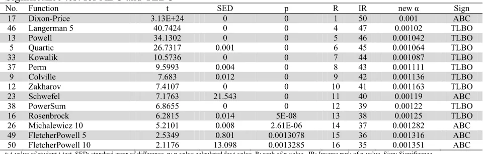
Table 7

Significance test for ABC and TLBO

No.

17 Dixon-Price 3.13E+24 0 0 1 50 0.001 ABC

46

Langerman 40.74245 0 0 474 0.00102 TLBO

13 Powell 34.1302 0 0 5 46 0.001042 TLBO

5

Quartic 26.7317 0.001 0 456 0.001064 TLBO

33 Kowalik 10.5736 0 0 7 44 0.001087 TLBO

37

Perm 9.5993 0.004 0 438 0.001111 TLBO

9 Colville 7.683 0.012 0 9 42 0.001136 TLBO

12

Zakharov 7.4107 0 100 41 0.001163 TLBO

23 Schwefel 7.1763 21.543 0 11 40 0.00119 ABC

38

PowerSum 6.8655 0 120 39 0.00122 TLBO

16 Rosenbrock 6.2815 0.014 5E-08 13 38 0.00125 TLBO

26

Michalewicz 5.210110 0.008 2.61E-06 14 37 0.001282 ABC

49 FletcherPowell 5 2.5349 0.801 0.0013078 15 36 0.001316 ABC

50

FletcherPowell 2.117610 13.098 0.0013285 16 35 0.001351 ABC

It is observed from Table 4 that for 28 functions TLBO is better than GA and on two functions GA is better than TLBO while for remaining 20 functions both the algorithms showed the equal performance. From Table 5, on 29 functions there is no significance difference between PSO and TLBO but on 20 functions TLBO is better than PSO while on one function PSO is better than TLBO. From Table 6, on 7 functions TLBO performed better than DE while on 4 functions DE is better than TLBO. On remaining 39 functions there is no significance difference between DE and TLBO. From Table 7, on 34 functions TLBO and ABC showed equal performance. On 11 functions, TLBO performed better than ABC while ABC performs better than TLBO on 5 functions.

3.2. Experiment 2

In this section, the performance of TLBO is compared with the different evolutionary algorithms like Canonical evolution strategies (CES), Fast evolution strategies (FES), Covariance matrix adaptation evolution strategies (CMA-ES) and Evolution strategies learned with automatic termination (ESLAT) along with the swarm intelligence based algorithm ABC. In this experiment the TLBO algorithm is implemented on 23 unconstrained benchmark functions taken from the previous work of Karaboga and Akay (2009). The details of the benchmark functions considered in this experiment are shown in Table 8. For the considered test problems, the TLBO algorithm is run for 50 times for each benchmark function. To maintain the consistency in the comparison between TLBO and other algorithms, in each run the algorithm is terminated when it has completed 100000 function evaluations or when it reached the global minima within the gap of 10-3_{. The results obtained using the TLBO algorithm are compared}

(13)

evaluations required for duplication removal considered are 2500, 5000, 7500 and 10000 for population sizes of 25, 50, 75 and 100 respectively when the maximum function evaluations of the algorithm is 100000.

Table 8

Benchmark functions considered in experiment 2 D: Dimension, C: Characteristic, U: Unimodal, M: Multimodal, S: Separable, N: Non-separable

No.

Function D Search _range No.C Function Search D range C

1 Sphere 30 [-100, 100] US 13 Penalized 2 30 [-50, 50] MN

2

Schwefel 302.22 [-10, UN10] 14 Fox holes [-65.536, 2 MS65.536]

3 Schwefel 1.2 30 [-100, 100] UN 15 Kowalik 4 [-5, 5] MN

4

Schwefel 302.21 [-100, UN100] 16 6 Hump camel back [-5, 2 MN5] 5 Rosenbrock 30 [-30, 30] UN 17 Branin 2 [-5, 0] × [10, 15] MS 6

Step 30 [-100, US100] 18 Goldstein-Price [-2, 2 MN2]

7 Quartic 30 [-1.28, 1.28] US 19 Hartman 3 3 [0, 1] MN

8

Schwefel 30 [-500, MS500] 20 Hartman 6 [0, 6 MN1]

9 Rastrigin 30 [-5.12, 5.12] MS 21 Shekel 5 4 [0, 10] MN

10

Ackley 30 [-32, MN32] 22 Shekel 7 [0, 4 MN10]

11 Griewank 30 [-600, 600] MN 23 Shekel 10 4 [0, 10] MN

12

Penalized 30 [-50, 50] MN

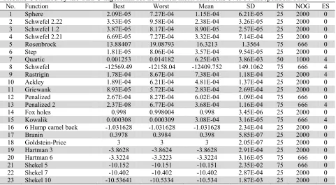
Table 9 shows the best results obtained using the TLBO algorithm along with its corresponding strategy.

Table 9

Results Obtained by the TLBO algorithm for 23 bench mark functions over 50 independent runs

No.

Function Best Worst Mean SD PS NOG ES

1 Sphere 2.09E-05 7.27E-04 1.15E-04 6.21E-05 25 2000 0

2

Schwefel 3.53E-052.22 9.58E-04 2.38E-04 3.26E-05 25 2000 0 3 Schwefel 1.2 3.87E-05 8.17E-04 8.90E-05 2.57E-05 25 2000 0 4

Schwefel 6.69E-052.21 7.27E-04 3.32E-04 7.14E-04 25 2000 0

5 Rosenbrock 13.88407 19.08793 16.3213 1.3564 75 666 0

6

Step 1.81E-05 8.06E-04 3.57E-04 9.54E-05 25 2000 0

7 Quartic 0.001253 0.014182 6.25E-03 3.86E-03 50 1000 4

8

Schwefel -12569.49 -12158.04 -12409.752 149.1062 75 666 4

9 Rastrigin 1.78E-04 8.67E-04 7.38E-04 1.18E-04 25 2000 4

10

Ackley 1.89E-04 6.21E-04 4.81E-04 1.37E-04 25 2000 0

11 Griewank 8.93E-05 5.72E-04 2.83E-04 2.69E-04 25 2000 0

12

Penalized 2.67E-04 8.27E-04 6.02E-04 1.09E-04 75 666 0 13 Penalized 2 2.37E-08 6.77E-04 3.68E-04 1.16E-04 75 666 4 14

Fox 0.998holes 0.998004 0.998 3.45E-06 25 2000 0

15 Kowalik 0.000308 0.000309 3.08E-04 3.16E-05 75 666 4

16 -1.0316286 Hump camel back -1.031628 -1.031628 2.34E-04 200025 0

17 Branin 0.3978 0.3984 0.398 5.85E-07 25 2000 0

18

Goldstein-Price 3 3 2.05E-073 25 2000 0

19 Hartman 3 -3.8628 -3.8624 -3.8628 2.91E-04 25 2000 0

20

Hartman -3.32246 -3.3223 -3.3224 3.16E-05 75 666 0

21 Shekel 5 -10.152 -10.151 -10.151 2.35E-02 75 666 0

22

Shekel -10.4027 -10.402 -10.402 2.87E-04 200025 0

23 Shekel 10 -10.53641 -10.5334 -10.534 1.87E-03 25 2000 0

(14)

Table 10

Comparative results of TLBO with other evolutionary algorithms over 50 independent runs

NO.

Function CES FES ESLAT CMA_ES ABC TLBO

Mean

SD Mean SD Mean SD Mean SD Mean SD Mean SD

1 Sphere 1.7E–26 1.1E–25 2.5E–04 6.8E–05 2.0E–17 2.9E–17 9.7E–23 3.8E–23 7.57E–04 2.48E–04 1.15E-04 6.21E-05 2

Schwefel 8.1E–20 2.22 3.6E–19 6.0E–02 9.6E–02 3.8E–05 1.6E–05 4.2E–11 7.1E–23 8.95E–04 1.27E–04 2.38E-04 3.26E-05 3 Schwefel 1.2 337.62 117.14 1.4E–03 5.3E–04 6.1E–06 7.5E–06 7.1E–23 2.9E–23 7.01E–04 2.78E–04 8.90E-05 2.57E-05 4

Schwefel 2.412.21 2.15 5.5E–03 6.5E–04 0.78 1.64 5.4E–12 1.5E–12 2.72 1.18 3.32E-04 7.14E-04

5 Rosenbrock 27.65 0.51 33.28 43.13 1.93 3.35 0.4 1.2 0.936 1.76 16.3213 1.3564

6

Step 0 0 0 2.0E–02 0 0.14 1.44 1.77 0 3.57E-040 9.54E-05

7 Quartic 4.7E–02 0.12 1.2E–02 5.8E–03 0.39 0.22 0.23 8.7E–02 9.06E–02 1.89E–02 6.25E-03 3.86E-03 8

Schwefel -8.00E+93 4.90E+94 -1.26E+04 3.25E+01 2.30E+15 5.70E+15 -7637.14 895.6 -12563.673 23.6 -12409.752 149.1062

9 Rastrigin 13.38 43.15 0.16 0.33 4.65 5.67 51.78 13.56 4.66E–04 3.44E–04 7.38E-04 1.18E-04

10

Ackley 6.0E–13 1.7E–12 1.2E–02 1.8E–03 1.8E–08 5.4E–09 6.9E–12 7.81E–04 1.83E–041.3E–12 4.81E-04 1.37E-04 11 Griewank 6.0E–14 4.2E–13 3.7E–02 5.0E–02 1.4E–03 4.7E–03 7.4E–04 2.7E–03 8.37E–04 1.38E–03 2.83E-04 2.69E-04 12

Penalized 1.46 3.17 2.8E–06 8.10E-07 1.5E–12 2.0E–12 1.2E–04 3.40E-02 6.98E–04 2.78E-04 6.02E-04 1.09E-04 13 Penalized 2 2.4 0.13 4.7E–05 1.5E–05 6.4E–03 8.9E–03 1.7E–03 4.5E–03 7.98E–04 2.13E-04 3.68E-04 1.16E-04 14

Fox 2.2holes 2.43 1.2 0.63 1.77 1.37 10.44 6.87 0.998 3.21E-04 0.998 3.45E-06

15 Kowalik 1.3E–03 6.3E–04 9.7E–04 4.22E–04 8.1E–04 4.1E–04 1.5E–03 4.2E–03 1.18E–03 1.45E-04 3.08E-04 3.16E-05 16 -1.0316 Hump camel back 1.2E–03 -1.0316 6.00E-07 -1.0316 9.7E–14 -1.0316 7.70E-16 -1.031 3.04E-04 -1.031628 2.34E-04 17 Branin 0.401 3.6E–3 0.398 6.00E-08 0.398 1.0E–13 0.398 1.40E-15 0.3985 3.27E-04 0.398 5.85E-07 18

Goldstein-Price 3.007 1.2E–02 3 0 5.8E–14 3 14.34 25.05 3.09E-043 2.05E-073

19 Hartman 3 -3.8613 1.2E–03 -3.86 4.00E-03 -3.8628 2.9E–13 -3.8628 4.80E-16 -3.862 2.77E-04 -3.8628 2.91E-04 20

Hartman -3.246 5.8E–2 -3.23 0.12 -3.31 3.3E–2 -3.28 5.8E–02 -3.322 1.35E-04 -3.3224 3.16E-05

21 Shekel 5 -5.72 2.62 -5.54 1.82 -8.49 2.76 -5.86 3.6 -10.151 1.17E-02 -10.151 2.35E-02

22

Shekel -6.097 2.63 -6.76 3.01 -8.79 2.64 -6.58 3.74 -10.402 3.11E–04 -10.402 2.87E-04

(15)

Table 11

Mean number of function evaluation (Mean FE) required by ESLAT, CMA-ES, ABC and TLBO algorithms for the benchmark functions considered in experiment 2

No. Function CES FES ESLAT CMA-ES ABC TLBO

Mean FE Mean FE Mean FE Mean FE Mean FE SD of FE Mean FE SD of FE 1 Sphere 69724 150,000 69724 10721 9264 1481 4648 148 2 Schwefel 2.22 60859 200000 60859 12145 12991 673 7395 163 3 Schwefel 1.2 72141 500000 72141 21248 12255 1390 12218 1305 4 Schwefel 2.21 69821 500000 69821 20813 100000 0 9563 715 5 Rosenbrock 66609 1500000 66609 55821 100000 0 100000 0 6 Step 57064 150000 57064 2184 4853 1044 13778 1491 7 Quartic 50962 300000 50962 667131 100000 0 100000 0

8 Schwefel 61704 900000 61704 6621 64632 23897 100000 0 9 Rastrigin 53880 500000 53880 10079 26731 9311 34317 13866 10 Ackley 58909 150000 58909 10654 16616 1201 3868 2634 11 Griewank 71044 200000 71044 10522 36151 17128 10090 16237 12 Penalized 63030 150000 63030 13981 73440 2020 10815 1430 13 Penalized 2 65655 150000 65655 13756 8454 1719 30985 12937 14 Fox holes 1305 10000 1305 540 1046 637 524 150 15 Kowalik 2869 400000 2869 13434 6120 4564 2488 2700

16 6 Hump 1306 10000 1306 619 342 109 447 175

17 Branin 1257 10000 1257 594 530 284 362 88

18 Goldstein-Price 1201 10000 1201 2052 15186 13500 452 244 19 Hartman 3 1734 10000 1734 996 4747 16011 547 135 20 Hartman 6 3816 20000 3816 2293 1583 457 24847 29465 21 Shekel 5 2338 10000 2338 1246 6069 13477 1245 114

22 Shekel 7 2468 10000 2468 1267 7173 9022 1272 99

23 Shekel 10 2410 10000 2410 1275 15392 24413 1270 135

Here the mean number of function evaluation indicates the function evaluations required to obtain global best solution within the gap of 10-3_{averaged over 30 independent runs.}

Table 12

Success rate of ESLAT, CMA-ES, ABC and TLBO algorithms for the benchmark functions considered in experiment 2

No. Function ESLAT CMA-ES ABC TLBO

1 Sphere 100 100 100 100

2 Schwefel 2.22 100 100 100 100

3 Schwefel 1.2 100 100 100 100

4 Schwefel 2.21 0 100 0 100

5 Rosenbrock 70 90 0 0

6 Step 98 36 100 100

7 Quartic 0 0 0 0

8 Schwefel 0 0 86 40

9 Rastrigin 40 0 100 100

10 Ackley 100 100 100 100

11 Griewank 90 92 96 100

12 Penalized 100 88 100 100

13 Penalized 2 60 86 100 100

14 Fox holes 60 0 100 100

15 Kowalik 94 88 100 100

16 6 Hump camel back 100 100 100 100

17 Branin 100 100 100 100

18 Goldstein-Price 100 78 100 100

19 Hartman 3 100 100 100 100

20 Hartman 6 94 48 100 96

21 Shekel 5 72 40 98 100

22 Shekel 7 72 48 100 100

23 Shekel 10 84 52 96 100

(16)

If for any function, the global best solution is not obtained in this precision then solution obtained in the last cycle is recorded. It is observed from the results that on 14 functions the computational effort of TLBO is less than the rest of the considered algorithms i.e. the convergence of TLBO is faster than rest of the algorithms. On 3 functions, ABC required minimum computational effort than the other algorithms. On 5 functions, CMA-ES and on 1 function ESLAT required less number of function evaluations to achieve the global best solution than rest of the considered algorithms. The success rate of all the algorithms for the considered benchmark functions are shown in Table 12.

It is observed from the results that ESLAT and CMA-ES achieved the best success rate on 9 functions while ABC and TLBO algorithms achieved the best success rate on 19 functions. On Schwefel and Hartman 6 functions ABC achieved higher success rate than TLBO while on Schwefel 2.21, Griewank, Shekel 5 and Shekel 10 functions success rate of TLBO is better than ABC. On Rosenbrock function success rate of CMA-ES is better than rest of the considered algorithms.

3.3. Experiment 3

In this section, the computational effort and consistency of the TLBO algorithm is compared with Self-organizing maps evolution strategy (SOM-ES), Neural gas networks evolution strategy (NG-ES), CMA-ES and ABC algorithms. In this experiment the TLBO algorithm is implemented on 3 unconstrained benchmark functions taken from the previous work of Karaboga and Akay (2009). The details of the benchmark functions considered in this experiment are shown in Table 13.

Table 13

Benchmark functions considered in experiment 3

No. Function Formulation D Search _range C

1 Modified _Rosenbrock

(

2

)

2 ( )2 ((11) (2 21 / 0.1)2 )

min 74 100 2 1 1 1 400exp

x x

F = + x −x + −x − − + + + 2 [-2, 2] UN 2 Modified Griewank

(

2 2

)

( )

min 1 2

1

1 cos cos

200 2

y F = + x +x − x ⎛_⎜ ⎞_⎟

⎝ ⎠ 2 [-100, 100] MN

3 Rastrigin 2

min 1

10cos(2 ) 10

D

i i

i

F x πx

=

⎡ ⎤

=

∑

_⎣ − + _⎦ ₂ _{[-5.12, 5.12] MS}

For the considered test problems, the TLBO algorithm is run for 10000 times for each benchmark function. In each run the maximum function evaluation is set as 5000 per test function. To maintain the consistency in the comparison, the limiting value of the satisfactory convergence is set as 40, 0.001 and 0.001 for functions 1, 2 and 3 respectively (Karaboga and Akay 2009, Milano et al. 2004). Here also

the TLBO algorithm is implemented with different combinations of population size, number of generation and elite size and the strategy which produced the best results is considered for the comparison.

(17)

Table 14

Comparative results of different algorithms for the benchmark functions considered in experiment 3

Algorithm Modified Rosenbrock Griewank Rastrigin

Mean FE % Success Mean FE % Success Mean FE % Success 5 × 5 SOM-ES 1600 ± 200 70 ± 8 130 ± 40 90 ± 7 180 ± 50 90 ± 7 7 × 7 SOM-ES 750 ± 90 90 ± 5 100 ± 40 90 ± 8 200 ± 50 90 ± 8 NG-ES (m=10) 1700 ± 200 90 ± 7 180 ± 50 90 ± 10 210 ± 50 90 ± 8 NG-ES (m=20) 780 ± 80 90 ± 9 150 ± 40 90 ± 8 180 ± 40 90 ± 7 CMA-ES 70 ± 40 30 ± 10 210 ± 50 70 ± 10 100 ± 40 80 ± 9 ABC 1371 ± 2678 52 ± 5 1124 ± 960 99 ± 1 1169 ± 446 100 ± 0 TLBO 1277 ± 942 62 ± 6 1164 ± 456 100 ± 0 1637 ± 596 100 ± 0

The TLBO algorithm has already been successfully applied by various researchers for solving complex benchmark functions and difficult engineering problems (Azizipanah-Abarghooee et al. 2012,

Hosseinpour et al. 2011, Krishnanand et al. 2011, Nayak et al. 2011, Niknam et al. 2012a, 2012b,

2012c, Rao and Kalyankar 2012a, 2012b, 2012c, Rao and Savsani 2012, Rao and Patel 2012a; 2012b; 2012c; 2012d, Satapathy and Naik 2011, Satapathy et al. 2012, Toğan 2012). Contrary to the opinion

expressed by Črepinšek et al. (2012) that TLBO is not a parameter-less algorithm, this paper has

clearly explained that TLBO is an algorithm-specific parameter-less algorithm and this was already stated by Rao and Patel (2012a). Common control parameters are common to run any of the optimization algorithms and algorithm-specific parameters are specific to the algorithm and different algorithms have different specific parameters to control. The TLBO algorithm does not have any algorithm-specific parameters to control and it requires only the control of the common control parameters like population size, number of generations and elite sizes. In fact, many of the comments made by Črepinšek et al. (2012) about the TLBO algorithm were already addressed by Rao and Patel

(2012a).

4. Conclusion

The tuning of the common controlling parameters such as population size and number of generations is one of the important factors in any probabilistic algorithm. In addition to this, evolutionary and swarm intelligence based algorithms require proper tuning of algorithm-specific parameters. A change in the tuning of the algorithm-specific parameters influences the effectiveness of the algorithm. The recently proposed TLBO algorithm does not require any algorithm-specific parameters. It only requires the tuning of the common controlling parameters of the algorithm for its working.

(18)

References

Ahrari, A. & Atai A. A. (2010). Grenade explosion method - A novel tool for optimization of multimodal functions. Applied Soft Computing, 10, 1132-1140.

Azizipanah-Abarghooee, R., Niknam, T., Roosta, A., Malekpour, A.R. & Zare, M. (2012). Probabilistic multiobjective wind-thermal economic emission dispatch based on point estimated method, Energy,

37, 322-335.

Basturk, B & Karaboga, D. (2006). An artificial bee colony (ABC) algorithm for numeric function optimization, in: IEEE Swarm Intelligence Symposium, Indianapolis, Indiana, USA.

Črepinšek, M., Liu, S-H & Mernik, L. (2012). A note on teaching-learning-based optimization algorithm, Information Sciences, 212, 79-93.

Dorigo, M., Maniezzo V. & Colorni A. (1991). Positive feedback as a search strategy, Technical Report 91-016. Politecnico di Milano, Italy.

Eusuff, M. & Lansey, E. (2003). Optimization of water distribution network design using the shuffled frog leaping algorithm. Journal of Water Resources Planning and Management, 29, 210-225.

Farmer, J. D., Packard, N. & Perelson, A. (1986).The immune system, adaptation and machine learning, Physica D, 22,187-204.

Fogel, L. J, Owens, A. J. & Walsh, M.J. (1966). Artificial intelligence through simulated evolution.

John Wiley, New York.

Geem, Z. W., Kim, J.H. & Loganathan G.V. (2001). A new heuristic optimization algorithm: harmony search. Simulation, 76, 60-70.

Hedar, A. & Fukushima, M. (2006). Evolution strategies learned with automatic termination criteria.

Proceedings of SCIS-ISIS 2006, Tokyo, Japan.

Holland, J. (1975). Adaptation in natural and artificial systems. University of Michigan Press, Ann

Arbor.

Hosseinpour, H., Niknam, T. & Taheri, S.I. (2011). A modified TLBO algorithm for placement of AVRs considering DGs, 26th International Power System Conference, 31st October – 2nd

November 2011, Tehran, Iran.

Karaboga, D. (2005). An idea based on honey bee swarm for numerical optimization, Technical Report-TR06, Computer Engineering Department. Erciyes University, Turkey.

Karaboga, D. & Akay, B. (2009). A comparative study of Artificial Bee Colony algorithm. Applied Mathematics and Computation, 214(1) 108-132.

Karaboga, D. & Basturk, B. (2007). A powerful and efficient algorithm for numerical function optimization: artificial bee colony (ABC) algorithm. Journal of Global Optimization, 39 (3), 459–

471.

Karaboga, D. & Basturk, B. (2008). On the performance of artificial bee colony (ABC) algorithm.

Applied Soft Computing, 8 (1), 687–697.

Kashan, A.H. (2011). An efficient algorithm for constrained global optimization and application to mechanical engineering design: League championship algorithm (LCA). Computer-Aided Design,

43, 1769-1792.

Kennedy, J. & Eberhart, R. C. (1995). Particle swarm optimization. Proceedings of IEEE International Conference on Neural Networks, IEEE Press, Piscataway, 1942-1948.

Krishnanand, K.R., Panigrahi, B.K., Rout, P.K. & Mohapatra, A. (2011). Application of multi-objective teaching-learning-based algorithm to an economic load dispatch problem with incommensurable objectives. Swarm, Evolutionary, and Memetic Computing, Lecture Notes in Computer Science 7076, 697-705, Springer-Verlag, Berlin.

Milano, M., Koumoutsakos, P. & Schmidhuber, J. (2004). Self-organizing nets for optimization. IEEE Transactions on Neural Networks, 2004, 15(3), 758-765.

(19)

Niknam, T., Fard, A.K. & Baziar, A. (2012a). Multi-objective stochastic distribution feeder reconfiguration problem considering hydrogen and thermal energy production by fuel cell power plants, Energy, 42, 563-573.

Niknam, T., Golestaneh, F., & Sadeghi, M.S. (2012b). θ-multiobjective teaching–learning-based optimization for dynamic economic emission dispatch. IEEE Systems Journal, 6, 341-352.

Niknam, T., Azizipanah-Abarghooee, R. & Narimani, M.R. (2012c). A new multi objective optimization approach based on TLBO for location of automatic voltage regulators in distribution systems. Engineering Applications of Artificial Intelligence,

http://dx.doi.org/10.1016/j.engappai.2012.07.004.

Passino, K.M. (2002). Biomimicry of bacterial foraging for distributed optimization and control. IEEE Control Systems Magazine, 22, 52–67.

Price K., Storn, R, & Lampinen, A. (2005). Differential evolution - a practical approach to global optimization, Springer Natural Computing Series.

Rao, R.V. & Kalyankar, V.D. (2012a). Parameter optimization of modern machining processes using teaching–learning-based optimization algorithm. Engineering Applications of Artificial Intelligence,

http://dx.doi.org/10.1016/j.engappai.2012.06.007.

Rao, R.V. & Kalyankar, V.D. (2012b). Multi-objective multi-parameter optimization of the industrial LBW process using a new optimization algorithm. Journal of Engineering Manufacture, DOI:

10.1177/0954405411435865

Rao, R.V. & Kalyankar, V.D. (2012c). Parameter optimization of machining processes using a new optimization algorithm. Materials and Manufacturing Processes, DOI:

10.1080/10426914.2011.602792

Rao, R.V. & Patel, V. (2012a). An elitist teaching-learning-based optimization algorithm for solving complex constrained optimization problems. International Journal of Industrial Engineering Computations, 3(4), 535-560.

Rao, R.V. & Patel, V. (2012b). Multi-objective optimization of combined Brayton and inverse Brayton cycle using advanced optimization algorithms, Engineering Optimization, doi:

10.1080/0305215X.2011.624183.

Rao, R.V. & Patel, V. (2012c). Multi-objective optimization of heat exchangers using a modified teaching-learning-based-optimization algorithm, Applied Mathematical Modeling,

doi:10.1016/j.apm.2012.03.043.

Rao, R.V. & Patel, V. (2012d). Multi-objective optimization of two stage thermoelectric cooler using a modified teaching-learning-based-optimization algorithm. Engineering Applications of Artificial Intelligence, doi:10.1016/j.engappai.2012.02.016

Rao, R.V. & Savsani, V.J. (2012). Mechanical design optimization using advanced optimization techniques. Springer-Verlag, London.

Rao, R.V., Savsani, V.J & Balic, J. (2012b). Teaching-learning-based optimization algorithm for unconstrained and constrained real-parameter optimization problems. Engineering Optimization,

http://dx.doi.org/10.1080/0305215X.2011.652103

Rao, R.V., Savsani, V.J. & Vakharia, D.P. (2011). Teaching-learning-based optimization: A novel method for constrained mechanical design optimization problems. Computer-Aided Design, 43 (3),

303-315.

Rao, R.V., Savsani, V.J. & Vakharia, D.P. (2012a). Teaching-learning-based optimization: A novel optimization method for continuous non-linear large scale problems. Information Sciences, 183 (1),

1-15.

Rashedi, E., Nezamabadi-pour, H. & Saryazdi, S. (2009). GSA: A gravitational search algorithm,

Information Sciences, 179, 2232-2248.

Runarsson, T.P. &Yao X. (2000) Stochastic ranking for constrained evolutionary optimization. IEEE Transactions on Evolutionary Computation, 4 (3), 284-294.

Satapathy, S.C. & Naik, A. (2011). Data clustering based on teaching-learning-based optimization.

Swarm, Evolutionary, and Memetic Computing, Lecture Notes in Computer Science 7077, 148-156,

(20)

Satapathy, S.C., Naik, A. & Parvathi, K. (2012). High dimensional real parameter optimization with teaching learning based optimization. International Journal of Industrial Engineering Computations, doi: 10.5267/j.ijiec.2012.06.001.

Simon, D. (2008). Biogeography-based optimization. IEEE Transactions on Evolutionary Computation, 12, 702–713.

Storn, R. & Price, K. (1997). Differential evolution - A simple and efficient heuristic for global optimization over continuous spaces. Journal of Global Optimization, 11, 341-359.

Toğan, V. (2012). Design of planar steel frames using teaching–learning based optimization,

Engineering Structures, 34, 225–232.

(21)

Appendix A: Code of Elitist TLBO algorithm for unconstrained problems

The code is similar to that given in Rao and Patel (2012a) for the constrained optimization problems. The files of TLBO, OUTPUT, AVG_RESULT, REMOVE DUPLICATE and RUNTLBO remain the same. However, the INITIALIZATION, IMPLEMENT and OBJECTIVE files of Rao and Patel (2012a) are to be replaced by the following files. To run the TLBO code, user has to create separate MATLAB files for each function (i.e. separate .m file for INITIALIZATION, IMPLEMENTATION, OBJECTIVE, etc.) and then the RUNTLBO file is to be executed.

%%%%%%%%%%%%%%%%%%%%%%%% INITIALIZATION %%%%%%%%%%%%%%%%%%%%%

function [Students, select, upper_limit, lower_limit, ini_fun, min_result, avg_result, result_fun, opti_fun, result_fun_new,

opti_fun_new] = Initialize(note1, obj_fun, RandSeed) format long;

select.classsize =25; select.var_num = 10; select.itration =100;

if ~exist('RandSeed', 'var')

rand_gen = round(sum(100*clock));

end

rand('state', rand_gen);

[ini_fun, result_fun, result_fun_new, opti_fun, opti_fun_new,] = obj_fun(); [upper_limit, lower_limit, Students, select] = ini_fun(select);

Students = remove_duplicate(Students, upper_limit, lower_limit); Students = result_fun(select, Students);

Students = sortstudents(Students); average_result = result_avg(Students); min_result = [Students(1).result]; avg_result = [average_result];

return;

%%%%%%%%%%%%%%%%%%%%%%% %%% IMPLEMENT %%%%%%%%%%%%%%%%%%%%%

function [ini_fun, result_fun, result_fun_new, opti_fun, opti_fun_new] = implement

format long;

ini_fun = @implementInitialize ; result_fun = @implementresult;

result_fun_new = @implementresult_new; opti_fun = @implementopti;

opti_fun_new = @implementopti_new;

return;

function [upper_limit, lower_limit, Students, select] = implementInitialize(select)

global lower_limit upper_limit ll ul

Granularity = 1; lower_limit = ll; upper_limit = ul;

ll =[-100 -100 -100 -100 -100 -100 -100 -100 -100 -100]; ul =[100 100 100 100 100 100 100 100 100 100]; upper_limit = ul;

for popindex = 1 : select.classsize for k = 1 : select.var_num

mark(k) =(ll(k))+ ((ul(k) - ll(k)) * rand); end

Students(popindex).mark = mark;

end

select.OrderDependent = true;

return;

function [Students] = implementresult(select, Students)

global lower_limit upper_limit

classsize = select.classsize;

for popindex = 1 : classsize for k = 1 : select.var_num

x(k) = Students(popindex).mark(k); end

(22)

end return

function [Studentss] = implementresult_new(select, Students)

global lower_limit upper_limit

classsize = select.classsize;

for popindex = 1 : size(Students,1) for k = 1 : select.var_num x(k) = Students(popindex,k); end

Studentss(popindex) = objective(x);

end return

function [Students] = implementopti(select, Students)

for i = 1 : select.classsize for k = 1 : select.var_num

Students(i).mark(k) = max(Students(i).mark(k), ll(k));

Students(i).mark(k) = min(Students(i).mark(k), upper_limit(k)); end

end

return;

function [Students] = implementopti_new(select, Students)

for i = 1 : size(Students,1) for k = 1 : select.var_num

Students(i,k)= max(Students(i,k), ll(k));

Students(i,k) = min(Students(i,k), upper_limit(k)); end

end

return;

%%%%%%%%%%%%%%%%%%%%%%%%% OBJECTIVE%%%%%%%%%%%%%%%%%%%%%%%

function yy=objective(x)

format long; for ikl=1 : 10 p(ikl)=x(ikl); end