SUBSURFACE CHARACTERIZATION USING HEAD-WAVE ARTIFACTS IN SEISMIC INTERFEROMETRY

(1)

ARTIFACTS IN SEISMIC INTERFEROMETRY

by

Thomas Dylan Mikesell

A dissertation

submitted in partial fulfillment of the requirements for the degree of

Doctor of Philosophy in Geophysics Boise State University

(2)

(3)

BOISE STATE UNIVERSITY GRADUATE COLLEGE

DEFENSE COMMITTEE AND FINAL READING APPROVALS

of the dissertation submitted by

Dissertation Title: Subsurface Characterization Using Head-Wave Artifacts in Seismic Interferometry

Date of Final Oral Examination: 2 December 2011

The following individuals read and discussed the dissertation submitted by student Thomas Dylan Mikesell, and they evaluated his presentation and response to questions during the final oral examination. They found that the student passed the final oral examination.

Kasper van Wijk, Ph.D. Chair, Supervisory Committee

John H. Bradford, Ph.D. Member, Supervisory Committee

Hans-Peter Marshall, Ph.D. Member, Supervisory Committee

Jodi L. Mead, Ph.D. Member, Supervisory Committee

Andrew Curtis, Ph.D. External Examiner

(4)

I have to express my gratitude to Dr. Kasper van Wijk for making my experience at Boise State University, and throughout our professional relationship, absolutely wonderful. I cannot describe how much I have enjoyed myself over the past four and half years. I attribute a lot of that enjoyment to Dr. van Wijk’s enthusiasm for research, and life in general. I would not trade this experience for the world. I would like to thank the members of the Physical Acoustics Lab, particularly Andy Lamb, Thomas Blum and Dr. Mila Adam for always giving input, reading abstracts and papers, and taking time from their busy schedules to make sure I had plenty of good meals, a fishing buddy, and other distractions.

Support for the work in this dissertation comes from multiple sources, but largely a Department of Defense National Defense Science and Engineering Graduate Fel-lowship and a National Science Foundation GK12 FelFel-lowship. I especially want to thank Dr. Karen Viskupic, Dr. David Wilkins, and Dr. Jim Belthoff for the GK12 opportunity. I learned a great deal about the importance of community outreach, and I am forever grateful for the knowledge I gained about myself and my role as an educator during my year as a GK12 fellow.

I thank my committee members, Dr. John Bradford, Dr. Hans-Peter Marshall, and Dr. Jodi Mead, for their interest in this dissertation as well as their time and

(5)

help with computer coding. I thank Dr. Alex Calvert for very stimulating talks about the virtual refraction theory during the beginning of this dissertation.

Developing a complete understanding of seismic interferometry was aided by a three month visit to Delft University of Technology, The Netherlands. I would par-ticularly like to thank Dr. Kees Wapenaar, Dr. Deyan Draganov, and Elmer Ruigrok, who put a lot of time and effort into making that trip possible, as well as helping bring me up to speed on all aspects of seismic interferometry.

Last but not least, I would like to thank friends and family, especially my parents Tom and Dana, my brother Jack, my sister Hannah, and her family–Stephen, Henry, and Wyatt. I feel extremely fortunate to have had the opportunity to return to Idaho for graduate school. Without their support, this experience would not have been so fun and enjoyable.

(6)

Seismologists continually work to improve images of the Earth’s interior. One new ap-proach is seismic interferometry, which involves cross-correlating the seismic wavefield recorded at two receivers to generate data as if one of the receivers was a source. Over the past decade, seismic interferometry has become an established technique to esti-mate the surface-wave part of the impulse response between two receivers; however, practical limitations in the source-energy distribution have made body-wave recovery difficult and causes spurious energy in the estimated impulse response. Rather than suppress such spurious energy, it can be useful to analyze coherent spurious events to help constrain subsurface parameters.

With this in mind, we examine a particular spurious event we call the virtual refraction. This event comes from cross-correlating head-wave (or critically refracted) energy at one receiver with reflection and refraction energy at the other receiver. For this particular spurious event, we find that, similar to surface waves, the important part of the source-energy distribution is readily available. The sources need to be at or past the critical offset from both receivers. In a horizontal, two-layer subsurface model, the slope of the virtual refraction defines the velocity of the fast layer (V2). Furthermore, the stationary-phase point in the correlation gather defines the critical offset, a property that depends on the thickness (H) and velocity (V1) of the slow

(7)

A two-layer numerical example is presented to illustrate the origin of the vir-tual refraction. After estimating the refractor velocity, a semblance analysis can be used to estimate H and V1. In field data from the Boise Hydrogeophysical Research Site, the virtual refraction alone is used to the estimate H, V1, and V2. This is an improvement over methods that rely on several wave types to fully characterize seismic properties above and below an interface. An exploration-scale active source seismic data set illustrates how we can use the method to build near-surface seismic models that can then be used for statics estimation in standard reflection process-ing. Finally, we investigate multi-component seismic interferometry for the virtual refraction, a technique that has recently been developed to more accurately estimate the surface-wave impulse response with higher signal-to-noise than traditional single component estimates. We find that using multi-component correlations to estimate shear wave virtual refractions also improves signal-to-noise, but with a dependence on the incidence angle of the incoming wavefield.

(8)

ACKNOWLEDGMENTS . . . iii

ABSTRACT . . . v

LIST OF FIGURES . . . xi

LIST OF TABLES . . . xix

1 INTRODUCTION . . . 1

1.1 Investigating Head Waves in Seismic Interferometry . . . 4

1.2 Characterizing an Aquifer with the Virtual Refraction . . . 4

1.3 Semblance Analysis on the Correlation Gather . . . 5

1.4 Statics Estimation with the Virtual Refraction . . . 6

1.5 Using the Green Tensor to Isolate Wave Modes . . . 6

2 INVESTIGATING HEAD WAVES IN SEISMIC INTERFEROMETRY . 8 2.1 A Two-Layer Model and the Interferometric Result . . . 9

2.2 Stationary Phase Analysis in the Far-Field . . . 11

2.3 Violation of the Far-Field Approximation . . . 13

2.4 A Line of Sources . . . 14

(9)

2.5 Conclusions . . . 19

3 CHARACTERIZING AN AQUIFER WITH THE VIRTUAL REFRACTION 20 3.1 Introduction . . . 21

3.2 2006 Field Seismic Data . . . 22

3.2.1 Data Acquisition . . . 22

3.2.2 The Virtual Shot Record . . . 26

3.2.3 Stationary-Phase Point . . . 27

3.3 2009 Field Seismic Data . . . 29

3.3.1 Data Acquisition . . . 29

3.3.2 The Virtual Shot Record . . . 30

3.3.3 Stationary-Phase Point . . . 31

3.4 Discussion . . . 33

4 SEMBLANCE ANALYSIS ON THE CORRELATION GATHER . . . 36

4.1 Introduction . . . 36

4.2 Velocity and Depth Estimation in the Cross-correlation Domain . . . 41

4.2.1 Numerical Data Example . . . 43

4.2.2 Stacking Semblance Panels . . . 43

4.3 Field Data Example . . . 46

(10)

5.2 Delay-Time Method . . . 56

5.3 The Modified Delay-Time Method in the Presence of Noisy Data . . . 62

5.4 Lateral Resolution and Model Accuracy . . . 66

5.6 Conclusion . . . 71

6 USING THE GREEN TENSOR TO ISOLATE WAVE MODES . . . 72

6.2 A Laboratory Experiment . . . 75

6.3 Rayleigh Wave Isolation with the Cross-Terms . . . 79

6.4 A Numerical Body Wave Experiment . . . 87

7 CONCLUDING REMARKS . . . 93

REFERENCES . . . 99

APPENDICES . . . 106

A THE REFRACTION TRAVEL TIME EQUATION . . . 106

A.1 The Tref r Derivation for a Two-Layered Model . . . 106

B SEMBLANCE ANALYSIS AND RESOLUTION . . . 109

B.1 Travel-Time Difference Equation . . . 109

(11)

B.3 Discussion . . . 113

C MULTI-COMPONENT CORRELATION GATHERS . . . 115

C.1 The Critical Offset . . . 116

D LIST OF CITING ARTICLES . . . 119

(12)

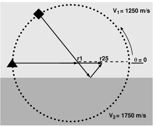
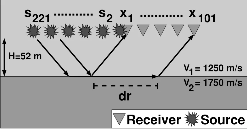
2.1 Layout of the acoustic numerical model with 2880 sources on a circle with radius 475 m and 101 receivers every 4 m on the dashed line, 52 m above the interface. Receiver r1 is located 75 m to the right of the circle center. The diamond and square infer stationary phase points, described in the section - The stationary phase in the far-field. 10 2.2 Left: shot record from an explosive source placed at receiver r1 (i.e.,

zero-offset) showing the direct, reflected, and refracted waves. Middle: virtual shot record based on a discretized Equation 2.1. The wavelet in the seismic interferometry result is the auto-correlation of the real shot wavelet. Right: correlation gather betweenr1 andr26 (dash line-middle plot) for all monopole sources on the top half of the circle. The stationary-phase regions are indicated with arrows and symbols correspond to those in Figure 2.1: the triangle is related to the direct wave, the diamond is related to the reflected wave. . . 11 2.3 Top: correlation gather between r1 and r101. Bottom: paths for

re-fracted waves traveling from source to r1 and r101. Note that these post-critical sources on the circle can be transposed to a line of sources. 15

(13)

addition to the direct, reflected, and refracted waves, we observe a lin-ear spurious event: the virtual refraction. Middle: virtual shot record for a line of explosive sources, showing direct and reflected waves, along with the virtual refraction. Right: correlation gather for r1 and r101 with a constant phase for the correlation between refracted waves at the larger offsets. Note also the stationary-phase point at the critical offset (dashed line) when the source is 106 m fromr1. . . 16 2.5 The ray path of reflection at the critical offset. . . 19

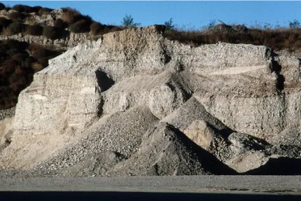
3.1 Quarry representative of BHRS geology showing: Sand Lenses, Poorly sorted massive units, moderately sorted horizontally bedded units, and trough crossbedded units. The vertical exposure is ∼6 m. . . 22 3.2 The P-wave velocity model representing the geology of the BHRS where

the 2006 survey was conducted. The elevation profile showing the 1 m dip was collected using a differential GPS. . . 23 3.3 Plan view of the BHRS. Survey geometry for the 2006 (red line) and

2009 (green line) 2D seismic lines at BHRS. Dashed line indicates the 1 m topographic dip in the 2006 line. We used variable spacing in the section where sources and receivers intersect in the 2009 line (described in detail in Section 3.3.1). The blue dots are the wells at the BHRS. . 25 3.4 a) Shot record for the source at S2. The data are filtered and gained. b)

Virtual shot record produced from seismic interferometry. The virtual refraction intercepts t=0 s at zero offset and has a velocity of 2700 m/s. 26

(14)

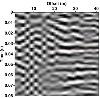
horizontal band at t ∼ 0.035 s (red dashed line) is caused by the correlation of refracted waves at both receivers. The correlation of reflected and refracted waves is not obvious with this source sampling so we cannot pick the stationary-phase point to get the critical offset. 28 3.6 a) Example shot record from source at S21. The data are filtered

and gained to suppress the groundroll and air wave. b) Virtual shot record produced by seismic interferometry. Note the virtual refraction intercepts t =0 s and has a velocity of 2700 m/s. R40 is the receiver correlated with R1 to produce the correlation gather in Figure 3.7. The virtual refraction arrives at R40 att ∼0.01 s. . . 30 3.7 Correlation gather of R1 and R40. The correlations of the refracted

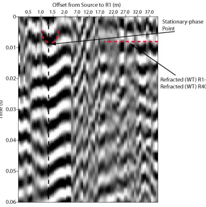
wave at R40 with the refracted and the reflected waves at R1 are highlighted in red. The critical offset (Xc) is denoted with the black

dashed line. Note the change in offset scale at 2 m. . . 32

4.1 Two-layer acoustic model with V1 = 1250 m/s, V2 = 1750 m/s and

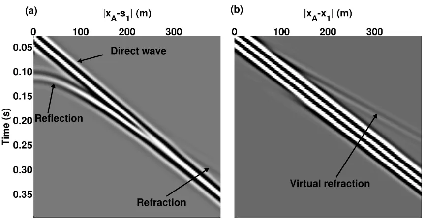
H = 52 m. The source increment is 2.5 m and receiver increment is 4 m. 38 4.2 Real shot record (a) and virtual shot record (b) for real and virtual

sources at s1 =x1. The virtual shot record contains the direct arrival and the virtual refraction artifact indicated by the arrow. . . 39 4.3 Correlation gather for |x101 −x1| = 400 m. The critical offset Xc

occurs at the maximum of Tdif f. Tc is the cross-correlation between

the refractions at both receivers and is equal to |x101_V−x1|

2 in this model. 40

(15)

(b), and |x101−x1|=400 m (c). As |xA−x1| increases, Tdif f becomes isolated in time and space. . . 44 4.5 Semblance panels for |x41−x1|=160 m (a),|x71−x1|=280 m (b), and

|x101−x1|=400 m (c). The star indicates the correct model parameters. 45 4.6 (a) Cross-correlation gather for |x101−x1| = 400 m. We add random

zero-mean Gaussian noise before cross-correlation so that Tdif f is no

longer visible. (b) Semblance panel for the cross-correlation gather. (c) Semblance panel after stacking 20 semblance panels from |x81−

x1|=320 m to |x101−x1|=400 m. . . 46 4.7 Boise Hydrogeophysical Research Site seismic model. Source and

re-ceiver spacing is 1 m. . . 47 4.8 (a) Trace-normalized shot record from a sledge-hammer source at the

first receiver location. (b) AGC and bandpass filtered shot record– dash indicates water table refraction. (c) Trace-normalized virtual shot record–dash indicates virtual refraction. . . 48 4.9 Sum of 30 semblance panels over the range of |x29 −x1|= 28 m to

|x59 −x1|=58 m. The white star denotes the maximum semblance, which occurs at 1.9 m and 395 m/s. The black start denotes the estimate from Chapter 3 and the dashed line indicates the water table depth from Johnson (2011). . . 50

(16)

and receiver (X1). Travel times are indicated along each ray path. For the travel path up from the interface receiverX1, the path is assumed the same from each side. . . 57 5.2 Synthetic model with varying surface layer thickness. Blue stars are

real sources and red stars are virtual sources. Green triangles represent receivers located at the surface. V1 and V2 are the constant compres-sional wave velocities in each layer. . . 58 5.3 Shot records for S1=500 m (a) and S2=1500 m (b). The first-break

picks are overlain in red. Receiver statics corrected shot records for

S1=500 m (c) andS2=1500 m (d) using the DT method. . . 59 5.4 (a) Combined arrival-time plot for first-break picks. (b) Receiver

stat-ics estimate from the DT method (red) compared to the true receiver statics (black). Dashed black lines indicate the crossover distance (Xd)

from each source. . . 61 5.5 Subsurface model with a receiver static under XA. To the left of the

blue line, the model does not impact the virtual refraction arrival time. 63 5.6 Shot records and first-break picks at S=500 and 1500 m after adding

zero-mean random Gaussian noise. . . 64 5.7 Virtual shot records for virtual sources at the red stars in Figure 5.2

(i.e., distance = 800 m (a) and 1200 m (b)). . . 64

(17)

(b) The MDT method receiver statics (red). The true static relative to zero elevation is the black line. The blue line shows the static estimated using the noisy data and DT method. The MDT method provides a superior result. . . 66 5.9 (a) Moveout of three wave types for sources at the edges of the receiver

array. (b) Moveout of the virtual refraction and direct wave for virtual shots at 800 m and 1200 m. Xc and Xd are the critical offset and

crossover distance, respectively. XVs is the virtual shot position. . . . 67 5.10 Comparison of the error estimate (σm) for each receiver. Black dashed

lines indicate the crossover distances (Xd) and dashed cyan lines

in-dicate the virtual shot positions. Error is reduced within the dashed lines because refractions exist in both forward and reverse directions. 69

6.1 Graphical presentation of relationships in Equation 6.3. Arrows indi-cate the source and receiver polarizations. . . 75 6.2 Laser ultrasonic laboratory experimental setup. A source laser

gen-erates an ultrasonic wavefield that is recorded at x0 and x by a laser interferometer. The model is a homogeneous piece of aluminum. This model represents a homogeneous halfspace at these wavelengths. . . . 77 6.3 Displacement in the vertical (z) and radial (r) directions recorded by

a laser interferometer at locations x0 and x shown in Figure 6.2. . . . 78

(18)

at x0 and x. (b) Comparison between cross-correlation of vertical-vertical with the difference between the signals in (a). (c) Hilbert transform of the difference in (a) compared to the vertical-vertical cross-correlation. . . 78 6.5 Location of the active stations in August of 2006 of the North line of

the Batholiths experiment. Red squares on the regional inset are BN01 and BN23. . . 80 6.6 Estimated Green tensor from cross-correlation of three days of ambient

noise. For the smaller station spacings in Gzz, an artifact at t ≈ 0 s interferes with the Rayleigh wave. In the lower right plot, Gc is red

and overlays Gzz (blue) in order to compare the presence or lack of

coherent energy at t≈0 s. . . 82 6.7 Summation of hourly f-k grids for the same three-day time window

used in the cross-correlations. Yellow triangles show station locations (distance scale on top and right). Dominant energy is from the West, with a secondary source of energy in the Southwest. . . 84 6.8 Top panel shows a comparison of the Green function estimates for three

stations. Bottom panels shows the waveform envelopes for each Green function above. For the smaller two station spacings, noise at t ≈0 s interferes with the Rayleigh-wave arrival inGzz (blue), but this artifact

is not present inGc(red). For wave fields with a large station spacings,

such as in the right panel, noise and signal are separated in time. . . 85

(19)

nents of the Rayleigh wave Green tensor. Gcshows significant improve-ment in coherency, particularly near 0.3 Hz. . . 86 6.10 Elastic numerical model used in multi-component seismic

interferome-try. The velocities areV1,P=1250 m/s,V1,S=400 m/s, V2,P=1750 m/s, V2,S=900 m/s. . . 87

6.11 (a) Vertical component zero-offset shot record. (b) and (c) vertical and radial component shot records, respectively, with added random Gaussian noise. . . 88 6.12 GZZ (a), GRR (b), GZR+RZ (c), and GZR−RZ (d) virtual shot records.

The first and last 10% of the source array is cosine tapered to zero before summing correlation gathers to generate the virtual shot record. 89 6.13 Comparison of amplitudes for different combinations of cross-correlations

at 65 m offset. The arrival is the virtual S wave. . . 90

A.1 Two-layer model and parameters used in derivation. . . 108

B.1 (a) 2D map of the semblance as a function of slow layer thickness and velocity. (b) 3D map of the semblance function. This display illustrates the steep sides around the peak. . . 111 B.2 Clipped semblance panels for minimum semblance values of 0.4 (a), 0.5

(b), 0.6 (c), 0.7 (d), 0.8 (e), 0.9 (f). The shape remains constant from b-f. . . 112

C.1 Raypath for a critically reflected wave and for a refracted PPP wave. 118

(20)

B.1 Table showing the deviation from the maximum semblance, normalized by the maximum semblance value. . . 113

(21)

CHAPTER 1:

INTRODUCTION

The field of seismology has changed tremendously over the past 50 years. Compu-tational power has expanded, as well as our ability to store large amounts of data. We have improved processing techniques and developed more accurate mathematical representations of the seismic wavefield. There have also been a number of advance-ments in hardware, such that we are able to record more broadband signals at a lower cost. In the end though, these improvements have all been made with one goal to improve the resolution and accuracy of seismic images.

(22)

(Wape-naar and Fokkema, 2006; Curtis et al., 2006). Seismic interferometry is a method to estimate the impulse response between any two receivers, as if one were a source. Two examples related to downhole receivers, where sources are extremely difficult to place, are given by Bakulin and Calvert (2006) and Mehta et al. (2007). Countless other studies have demonstrated that seismic interferometry is a technique that can improve the spatial sampling of seismic surveys for many geometries. In principle, at the exploration scale, this allows one to increase stacking fold cheaply while avoiding sources in sensitive areas where dynamite and vibroseis are not appropriate. It also allows us to redatum the wavefield, eliminating difficult statics problems caused by the complex near-surface.

The major requirement of seismic interferometry is that the wavefield be recorded simultaneously at both receivers. If this is the case, the method can even be applied to passive-source seismic data. Previously, passive seismologists were limited to using the impulse response between a receiver and an earthquake. Unfortunately, earthquakes occur mostly near plate boundaries, limiting subsurface illumination in some parts of the Earth. Ambient noise tomography, which has added a new dimension to surface-wave inversion for the Earth’s lithosphere, is closely related to seismic interferometry. Using Earth’s natural seismic noise (e.g., ocean microseism), we can now estimate phase- and group-velocity dispersion curves between distributed station pairs and invert for 3D velocity structure (e.g., Sabra et al., 2005; Shapiro et al., 2005; Lin

et al., 2008; Ekstrom et al., 2009). This approach greatly improves our ability to

illuminate the subsurface, as well as allows us to turn earthquakes into receivers buried deep within the Earth (Curtis et al., 2009).

(23)

comes from all directions. In passive-source seismology, this is called the equipartition of waves and often comes from multiple scattering. Equipartition means that all directions of propagation are equally likely (i.e., the wavefield has no preferred wave number). In active-source seismology, we need to place sources everywhere, or at least everywhere in the subsurface surrounding the two receivers (Wapenaar and Fokkema, 2006). In either case, it has been known for many years that the sources everywhere

requirement can be relaxed as long as the stationary-phase points in the seismic interferometry integral are sampled.

(24)

1.1 Investigating Head Waves in Seismic

Interferometry

This chapter covers the application of seismic interferometry to a two-layer acoustic model. The majority of this chapter was published as Mikesellet al.(2009). It begins with a short introduction to seismic interferometry and critically refracted (i.e., head wave) energy. Using an active-source numerical example, we illustrate how head waves behave during the application of seismic interferometry. Specifically, we highlight an artifact in the interferometric wavefield due to violating the theoretical restrictions placed on seismic interferometry. This artifact is the virtual refraction.

1.2 Characterizing an Aquifer with the Virtual

Refraction

(25)

cross-correlation of wavefields recorded at two receivers for all sources. A stationary-phase point associated with the correlation between the reflected wave and refracted wave from the interface identifies the critical offset. By combining information from the virtual shot record, the correlation gather, and the real shot record, we determine the seismic velocities of the unsaturated sand, as well as the relative depth to the water table. This work demonstrates the requirements placed on spatial sampling in order to recover information about the subsurface using the virtual refraction.

1.3 Semblance Analysis on the Correlation

Gather

(26)

1.4 Statics Estimation with the Virtual

Refraction

In this chapter, we apply the virtual refraction analysis to 2D synthetic land seismic exploration data with statics caused by near-surface weathering layer thickness vari-ations. Using the delay-time method, we estimate source and receiver statics using first-break arrival times. We go on to develop a modified delay-time method, wherein we use the first-break arrival times of the virtual refraction to isolate and estimate re-ceiver statics. We show that this approach simplifies the inverse problem by removing the source static term from the delay-time equation. Finally, we show that using the virtual refraction extends lateral resolution and is better suited for estimating statics when the data are noisy.

1.5 Using the Green Tensor to Isolate Wave

Modes

(27)

(28)

CHAPTER 2:

INVESTIGATING HEAD WAVES IN SEISMIC

INTERFEROMETRY

Summary

(29)

2.1 A Two-Layer Model and the Interferometric

Result

Consider the two-layer acoustic model shown in Figure 2.1. The top layer has velocity

V1 = 1250 m/s, the bottom layer has velocity V2 = 1750 m/s, and the density is 1000 g/cm3 _{in both layers. We place an explosive seismic source (with a dominant} wavelength of ∼30 m) at the first receiver location (r1) and model the wavefield for 0.8 s after the explosion on 101 receivers evenly spaced on a 400 m line, 52 m above the interface. We use the spectral element modeling method, widely used in global seismology (Komatitsch and Vilotte, 1998; Komatitsch and Tromp, 2002). The left panel of Figure 2.2 shows three coherent events in the modeled wave field: 1) the direct wave, 2) the reflected wave from the interface, and 3) the refracted wave at offsets greater than 300 m. Now, using seismic interferometry, we attempt to recover the wavefield between two receiver positions based on Equation 19 from Wapenaar and Fokkema (2006), which represents the exact acoustic Green’s function:

ˆ

G(xA,xB) + ˆG∗(xA,xB) =

I

S

−1

jωρ(x)( ˆG

∗

(xA,x)∂i( ˆG(xB,x))

− ∂i( ˆG∗(xA,x)) ˆG(xB,x))nidS, (2.1)

where ˆG(xA,xB) denotes the causal frequency domain Green’s function at xAfrom a

source at xB and ˆG∗(xA,xB) denotes the complex conjugate Green’s function, which

corresponds to the anticausal time-domain Green’s function. Angular frequency is ω,

ρis density andj is√−1. ˆG∗(xA,x) and ˆG(xB,x) represent the Green’s functions at

locationsxA and xB due to a monopole source atx, and∂iGˆ∗(xA,x) and∂iGˆ(xB,x)

(30)

r25 _θ

V = 1750 m/s

r1 _{= 0}

V = 1250 m/s₁

2

Figure 2.1: Layout of the acoustic numerical model with 2880 sources on a circle with radius 475 m and 101 receivers every 4 m on the dashed line, 52 m above the interface. Receiver r1 is located 75 m to the right of the circle center. The diamond and square infer stationary phase points, described in the section - The stationary phase in the far-field.

x. S is the closed integration surface around the receivers xA,B. To approximate

this analytic result, we use a finite number of sources on a surface surrounding our receivers (Figure 2.1). We choose the integration surface S to be a circle with radius 475 m. We place the receiver array 75 m to the right of the circle center. We distribute 2880 dipole and monopole seismic sources evenly over the circle, approximately one dipole and monopole source every meter along the circle. We simulate a monopole source using an explosive source. A dipole source consists of the addition of an explosion (located 2.5 m outside the circle) and an implosion (located 2.5 m inside the circle), divided over the distance (5 m) between them. We center the dipole at the monopole source location and orient it normal to the circle.

(31)

po-0 0.05 0.10 0.15 0.20 0.25 0.30 Time (s)

0 100 200 300 400

Offset (m) Direct wave Refracted wave Reflected wave 0 0.05 0.10 0.15 0.20 0.25 0.30 Time (s)

0 100 200 300 400 Offset (m)

r26 Direct wave

Noise

Refracted wave

Reflected wave

0 0.03 0.05 0.08 0.10 0.12 0.15 0.18 Time (s)

0 30 60 90 120 150 Angle ( )o

Direct r1 − Direct r26

Direct r1 − Reflected r26

Figure 2.2: Left: shot record from an explosive source placed at receiverr1 (i.e., zero-offset) showing the direct, reflected, and refracted waves. Middle: virtual shot record based on a discretized Equation 2.1. The wavelet in the seismic interferometry result is the auto-correlation of the real shot wavelet. Right: correlation gather between r1 and r26 (dash line-middle plot) for all monopole sources on the top half of the circle. The stationary-phase regions are indicated with arrows and symbols correspond to those in Figure 2.1: the triangle is related to the direct wave, the diamond is related to the reflected wave.

sition. We set xB = r1 so that it is always this receiver cross-correlated with the

101 receivers; r1 is commonly called the virtual source (Bakulin and Calvert, 2004). After summing the cross-correlations for all sources, we obtain the virtual shot record shown in the middle panel of Figure 2.2. Because we are limited to a finite number of sources on S, we observe some noise before the first breaks. There is a phase differ-ence in the source wavelet between the real and the virtual shot records because the source wavelet is squared in the cross-correlation procedure of seismic interferometry (Snieder, 2004; Wapenaar and Fokkema, 2006).

2.2 Stationary Phase Analysis in the Far-Field

(32)

• All sources lie in the far-field (i.e., the distance from the source to the receivers and scatterers is large compared to the wavelength).

• Rays take off approximately normal from the integration surface S.

• The medium outside the integration surface S is homogeneous, such that no energy going outward from the surface is scattered back into the system.

• The medium around the source is locally smooth (the high-frequency approxi-mation).

Following these assumptions, the spatial derivative can be approximated by a time derivative:

∂iGˆ(xA,x)ni ≈ −j ω c(x)

ˆ

G(xA,x). (2.2)

With this approximation, Equation 2.1 simplifies to Equation 31 in Wapenaar and Fokkema (2006):

ˆ

G(xA,xB) + ˆG∗(xA,xB)≈

I

S

2 ˆG∗(xA,x) ˆG(xB,x)

ρ(x)c(x) dS, (2.3)

where c is the acoustic velocity. From this expression, we use the stationary phase argument (e.g., Snieder, 2004) to investigate the origin of events in the virtual shot record. In the right panel of Figure 2.2, we present the causal part of the correlations between r1 and r25 (i.e., offset |xA −xB| = 100 m) for all monopole sources in

(33)

coherent events in this so-called correlation gather that give rise to the events in the virtual shot record (Mehtaet al., 2008). The correlation of the direct wave atr1 with the direct wave at r25 has a stationary phase point at 180◦ and is associated with the direct wave traveling from r1 tor25 in ∼0.08 s. The arrows marked with a black triangle in Figure 2.1 and in the right panel of Figure 2.2 indicate that this is the source location where source and receiver are in-line. Another coherent event in the virtual shot record stems from the correlation between the direct wave at receiver r1 and the reflected wave at r25. This event has a stationary phase point at ∼ 120◦ associated with the reflected wave traveling from r1 to r25 in ∼ 0.12 s. The arrows marked with a black diamond in Figure 2.1 and in the right panel of Figure 2.2 indicate that this is the source location where the wave reflects to r25 after passing through r1. These stationary phase points result in the two arrivals in the middle panel of Figure 2.2 at 100 m offset. The weaker correlations seen at sources past 150◦ are associated with refractions and are discussed next.

2.3 Violation of the Far-Field Approximation

(34)

the correlation is only a function of the difference in travel paths along the refractor, denoted by dr in the bottom panel of Figure 2.3. As we show next, this correlation does not cancel when using only explosive (i.e., monopole) sources required by the approximate interferometric integral.

The virtual shot record using the approximate far-field integral (i.e., using only monopole sources on the circle) is shown in the left panel of Figure 2.4. Again we recover the correct direct, reflected, and refracted waves. However, we also observe a spurious linear event traveling at V2 = 1750 m/s going through the origin. We call this spurious arrival the virtual refraction. This event is a direct result of violating the far-field approximation represented by Equation 2.2, as it is the only approximation we made to the exact interferometric integral. The assumptions in Equation 2.2 are violated for those sources where the interface between V1 and V2 is located in the near-field.

2.4 A Line of Sources

(35)

0.10

0.12

0.15

0.18

0.20

0.23

Time (s)

140 150 160 170 180

Angle ( )

Reflected r1 − Refracted r101

Direct r1 − Refracted r101

o

Refracted r1 − Refracted r101

dr

r101

r1

2 1

Line of sources

V

(36)

0 0.05 0.10 0.15 0.20 0.25 0.30 Time (s)

0 100 200 300 400

Offset (m) Reflected wave Refracted wave Virtual refraction Direct wave 0 0.05 0.10 0.15 0.20 0.25 0.30 Time (s)

0 100 200 300 400

Offset (m)

Virtual refraction Reflected wave

Direct wave Truncation phase 0.10

0.15

0.20

0.25

Time (s)

100 200 300 400 500 Offset from source to r1 (m)

Stationary point

Figure 2.4: Left: virtual shot record using only explosive sources on the circle. In addition to the direct, reflected, and refracted waves, we observe a linear spurious event: the virtual refraction. Middle: virtual shot record for a line of explosive sources, showing direct and reflected waves, along with the virtual refraction. Right: correlation gather for r1 andr101 with a constant phase for the correlation between refracted waves at the larger offsets. Note also the stationary-phase point at the critical offset (dashed line) when the source is 106 m from r1.

obtained following Equation 2.3 using the line of explosive sources. We identify the direct, reflected, and refracted waves, as well as the virtual refraction. Other linear events not crossing the origin are truncation phases, as our source coverage is abruptly ended on each side of the source line (Snieder et al., 2008). The small amplitude variations in the virtual refraction at ∼ 0.15 s and ∼ 0.25 s arise from wave interference with these truncation phases. It is worth noting that because all contributions from post-critical sources sum constructively, the virtual refraction is robust in the presence of uncorrelated noise.

2.4.1 The Critical Offset

(37)

definitiont= 0 s. Therefore, unlike in conventional refraction analysis (Palmer, 1986; Lowrie, 2007), important subsurface information about the top-layer velocity V1 and interface depth H cannot be determined from the virtual refraction alone. Despite this, Tatanova et al. (2009, 2011) have shown that time-lapse measurements of the virtual refraction are useful for reservoir monitoring.

We overcome the lack of a refraction intercept time by investigating events in the correlation gather between r1 and r101 for the line of explosive sources (right panel of Figure 2.4). For long offset sources, we see the constant feature att ≈0.23 s. The correlation between the direct and the refracted wave is represented by a straight line while the curving feature represents the correlation between the reflected and refracted waves, having an extremum at x ≈ 106 m (dashed line). This stationary-phase point, associated with the correlation between reflected and refracted waves, occurs at the critical offset.

Using the sine of the critical angle sin(θc)≡V1/V2, Pythagorean theorem, and the parameters in Figure 2.5, we write

sin(θc)≡ V1

V2

= _q Xc/2 (Xc/2)

2 +H2

⇔Xc=

2V1H

p

V2 2 −V12

. (2.4)

(38)

the difference in arrival times to zero and solve for offset x:

d

dx(tref r−tref l) = 0 ⇔ d

dx

 

2Hcosθc V1 + x V2 − s x V1 2 + 2H V1 2 

= 0 ⇔

1

V2

− x

V1

q

x2_{+ (2}_H₎2

= 0 ⇔ x= _p2V1H

V2 2 −V12

, (2.5)

which equals the definition of the critical offset in Equation 2.4. The critical time

tc can be picked on real data as the arrival time of the reflected event on r1 for the

source at Xc ≈ 106 m. Then, with observables xc, tc, and V2, we can uniquely solve for H by rearranging Equation 2.4:

H =Xc

q

V2

2 −V12/(2V1). (2.6)

Usingtc = 2pH2_{+ (}_Xc/₂₎2_/V

1 and Equation 2.6, we can also solve for the top-layer wave speed V1:

V1 =

p

(V2Xc)/tc. (2.7)

(39)

X

1

2 H

c

θ

V

Figure 2.5: The ray path of reflection at the critical offset.

2.5 Conclusions

(40)

CHAPTER 3:

CHARACTERIZING AN AQUIFER WITH THE

VIRTUAL REFRACTION

Summary

(41)

3.1 Introduction

(42)

Figure 3.1: Quarry representative of BHRS geology showing: Sand Lenses, Poorly sorted massive units, moderately sorted horizontally bedded units, and trough cross-bedded units. The vertical exposure is ∼6 m.

develop the seismic velocity model shown in Figure 3.2.

3.2 2006 Field Seismic Data

3.2.1 Data Acquisition

(43)

Unsat. Sediments - v1=400 m/s

Sat. Sediments - v2=2700 m/s

Unknown Layer - v3= 2150 m/s

(silt or clay) Red Clay - v3=1700 m/s

Deep layer - v4= ?

0

?

D

epth (m)

R74 S/R1

(1 m spacing)

S20 _{(2 m spacing)}

H

v₁

v₀

70

v₃

v₄

20

dr

v₂

(44)

(45)

(46)

Noise

Virtual refraction

Pull−up

Residual air wave

a) b)

t

0

Figure 3.4: a) Shot record for the source at S2. The data are filtered and gained. b) Virtual shot record produced from seismic interferometry. The virtual refraction intercepts t=0 s at zero offset and has a velocity of 2700 m/s.

3.2.2 The Virtual Shot Record

Following Equation 2.3, we cross-correlate wavefields recorded at receiver R1 with wavefields recorded at receivers R1 to R74, for shots at positions S1 to S20. Sum-ming the cross-correlations for all 20 sources produces a virtual shot at receiver R1 (Figure 3.4b). While this is an elastic medium, we only record the vertical compo-nent of the wavefield, and consider only the pure P-wave refraction. Therefore, it is kinematically equivalent to the acoustic numerical example shown in Chapter 2.

(47)

the virtual shot record. The virtual refraction always intercepts zero offset at zero time. Therefore, it is relatively straightforward to pick the virtual refraction on the virtual shot record. Additionally, the uncorrelated noise before the refraction has been suppressed due to the summation over sources in seismic interferometry.

3.2.3 Stationary-Phase Point

Figure 3.5 shows the correlation gather for receivers R1 and R74 for S1 to S20. We observe the correlation of the refracted wave at R1 and the refracted wave at R74 at t ∼ 0.035 s for large offsets. While we see the constant correlation between both refracted waves for large-offset sources, we do not see the stationary-phase point from the correlation of the refracted wave at R74 with the reflected wave at R1, as we do in the numerical data (right panel of Figure 2.4). Since we do not observe the stationary-phase point in the correlation gather, we do not know Xc. This in turn

prevents the determination of V1 and H using Equations 2.7 and 2.6, respectively. Instead, we calculate the critical offset using our model values:

θc= arcsin

V2

V1

= arcsin

400 2700

= 8.5⇐ (3.1)

Xc= 2Htan (θc) = 8 tan (8.5o) = 1.2 m.

(48)

(49)

3.3 2009 Field Seismic Data

3.3.1 Data Acquisition

In May 2009, we designed and conducted a second 2D seismic survey at the Boise Hydrogeophysical Research Site (BHRS). The survey line was 86 m long, located on horizontal ground near the 2006 survey (Figure 3.3). We recorded on 91 variably spaced 100 Hz vertical-component geophones. The variable spacing gave better reso-lution near the critical offset while allowing us to record greater offsets. There were 74 receivers with 1 m spacing. On the end nearest the sources, we placed 17 receivers with 0.25 m spacing. Our source was a 4 lb. sledge hammer. Starting at the first receiver, we stacked 4 shots every 0.1 m for the first 2 m, while moving away from the receiver array. We then increased the shot spacing to 1 m, for another 38 m. We recorded for 0.5 s with a sampling interval of 0.25 ms.

(50)

a) b)

R40

Figure 3.6: a) Example shot record from source at S21. The data are filtered and gained to suppress the groundroll and air wave. b) Virtual shot record produced by seismic interferometry. Note the virtual refraction interceptst=0 s and has a velocity of 2700 m/s. R40 is the receiver correlated with R1 to produce the correlation gather in Figure 3.7. The virtual refraction arrives at R40 at t∼ 0.01 s.

3.3.2 The Virtual Shot Record

(51)

3.3.3 Stationary-Phase Point

We change to a trapezoidal bandpass filter with corner frequencies 30-75-150-300 Hz. This reduces the ringyness and emphasizes the cross-correlation of the refracted wave with the reflected wave from the water table in the correlation gather. By cross-correlating wavefields from R1 and R40 for all sources, we create a correlation gather (Figure 3.7). The correlation gather has a variable scale along the horizontal axis to highlight the stationary-phase point. We observe the stationary-phase point from the correlation of the water table reflection at R1 and the water table refraction at R40 at Xc =1.3 m. We also observe the flat feature at far offsets, at t ∼0.01 s resulting

from the correlation of the refracted wave at R1 and the refracted wave at R40. The lack of coherency between 5 m and 22 m offsets is caused by correlations involving residual groundroll not completely remove by the bandpass filter.

We know V2 =2700 m/s from the virtual shot record. We can use the real shot record to pick the critical time Tc =0.0185 s at Xc. Using Equations 2.7 and 2.6,

we find that V1 =440 m/s and H =3.9 m. For comparison, a conventional refraction analysis requires the intercept time and the upper and lower layer velocities to esti-mate H. Looking back to the real shot record with a source at the first receiver, we estimate the refraction intercept time is Ti =0.018 s. Because we do not observe the

direct wave, we useV1 =440 m/s (Moretet al., 2004). The velocity of the faster layer

V2 =2700 m/s can be estimated from the slope of the real refraction. Calculating the depth to interface using (Equation 3-41a in Yilmaz, 2001):

H = V1V2Ti 2pV2

2 −V12

(52)

Figure 3.7: Correlation gather of R1 and R40. The correlations of the refracted wave at R40 with the refracted and the reflected waves at R1 are highlighted in red. The critical offset (Xc) is denoted with the black dashed line. Note the change in offset

(53)

yieldsH =4.0 m. Traditional and interferometric refraction analysis are in agreement. We note that the virtual refraction method does not explicitly need an estimate ofV1, but both traditional and interferometric methods require user interpretation to pick the values going into estimates of V1 and H. In the example shown here, V1 matches well with Moretet al.(2004), but H is slightly larger than estimates using an electric tape measurement (Johnson, 2011) near the time of data collection. This is analyzed in the next chapter.

3.4 Discussion

(54)

sources produced similar quality virtual shot records due to the summing involved in seismic interferometry.

Another factor contributing to effective use of the virtual refraction method is the preprocessing. For the data used in this work, we found that a bandpass filter and an automatic gain control (AGC) best emphasized the refraction while minimizing the groundroll and other near-surface effects. The goal of our preprocessing was to emphasize the reflected and refracted wave from the desired interface. Because our interface was very shallow we found that more aggressive filtering of the groundroll reduced the correlation between the reflected and refracted waves from the water table. Another option to highlight the reflection and refraction would be time win-dowing. By windowing around the reflected wave at R1, only the correlations with the reflected wave would be present in the virtual shot record and correlation gather (Bakulin and Calvert, 2006). While windowing may help, it would be difficult be-cause we are not able to identify the reflection in the real shot record. However, we are able to observe the virtual refraction in the virtual shot and the correlations in the correlation gather without applying manual mutes.

3.5 Conclusions

(55)

(56)

CHAPTER 4:

SEMBLANCE ANALYSIS ON THE

CORRELATION GATHER

Summary

In Chapter 3, we used an artifact in seismic interferometry related to critically re-fracted waves that allowed us to determine the velocity of the refracting layer. In this chapter, we present a new semblance analysis on the cross-correlation of reflection and refraction energy to estimate the depth and velocity of the slow layer, without the need for manually picking the critical offset in the correlation gather. We illustrate this concept by a numerical example and show that it more accurately describes the water table depth in field data from the Boise Hydrogeophysical Research Site.

4.1 Introduction

(57)

re-ceivers. In the far-field approximation, the sum of the frequency-domain Green’s function G and the complex conjugate G∗ between two stations positioned at xA

and xB is shown in Equation 2.3. This is commonly referred to as the seismic

in-terferometric integral. With the survey geometry illustrated in Figure 4.1, we model the acoustic wavefield for 221 40-Hz Ricker wavelet sources at a 2.5 m interval using the spectral element method (Komatitsch and Vilotte, 1998; Komatitsch and Tromp, 2002). We record the wavefield at 101 receivers spaced 4 m apart. This is a similar numerical experiment as in Chapter 2. The difference here is the notation used as a consequence of the aforementioned semblance method.

The correlation gather is herein defined as the cross-correlations between xA and

xB for all sources, and summing the correlation gather for each receiver xA, we

generate a virtual shot record (Mehta et al., 2008) as though there was a source at

xB. In Chapter 2, we use this model to show that when sources are not in the

far-field and do not enclose the receivers, the retrieved virtual shot record contains an artifact related to critically refracted waves. We now use the same model to show an automated approach to characterizing a two-layer subsurface model.

Following Equation 2.3, we cross-correlate every receiver record in the array with the record at xB =x1, the receiver colocated at s1. Figures 4.2(a) and 4.2(b) show the real and virtual shot records for this model, respectively. The x-axes represent the distance between the real or virtual source at s1 = x1 and a given receiver at

xA. In Figure 4.2(b), we retrieve the direct-wave arrival from the cross-correlation

(58)

Source

Receiver

x

1 ...

x

101 dr

s

2

1 V = 1250 m/s

V = 1750 m/s

2 H=52 m

s

221 ...

Figure 4.1: Two-layer acoustic model with V1 = 1250 m/s, V2 = 1750 m/s and

H = 52 m. The source increment is 2.5 m and receiver increment is 4 m.

is produced because of an incomplete source distribution and the far-field radiation approximation inherent within Equation 2.3. The most intuitive reason for the virtual refraction is that cross-correlations of refractions from sources past the critical offset fromx1 (Figure 4.1) sum constructively during seismic interferometry. This energy is constant across the source array (e.g., Tc in Figure 4.3), and therefore, does not sum destructively when summing the cross-correlations over all sources.

(59)

Virtual refraction

Refraction Reflection

(b) (a)

Direct wave

Figure 4.2: Real shot record (a) and virtual shot record (b) for real and virtual sources ats1 =x1. The virtual shot record contains the direct arrival and the virtual refraction artifact indicated by the arrow.

produced from the incomplete source aperture (Snieder et al., 2006).

In conventional refraction analysis, we estimate V1 and V2 from the slope of the direct and refracted waves, respectively, and estimate the depth to the interface using Equation 3.2. The virtual refraction, on the other hand, has an intercept time Ti =

0 s. Therefore, in Chapter 3, we extracted H and V1 by estimating V2 from the moveout of the virtual refraction and picking the critical offset (Xc) in the

cross-correlation gather. However, estimating Xc manually can prove difficult in noisy

(60)

Figure 4.3: Correlation gather for |x101−x1| = 400 m. The critical offset Xc occurs at the maximum of Tdif f. Tc is the cross-correlation between the refractions at both

receivers and is equal to |x101_V−x1|

(61)

wave mask the direct wave and the shallow water table reflection.

4.2 Velocity and Depth Estimation in the

Cross-correlation Domain

We propose a semblance method of the correlation gather to estimate V1 and H, similar to King et al. (2011) and Poliannikov and Willis (2011), but focused on the virtual refraction. Figure 4.3 shows the correlation gather for |x101 −x1| = 400 m for all sources in Figure 4.1. The cross-correlation between the reflection at xB and

the refraction at xA yields Tdif f. We annotate the curve Tdif f in Figure 4.3 as well

as indicate the critical offset,Xc, and the cross-correlation between the refractions at

both receivers, Tc.

For a linear source array, we showed in Chapter 2 that the maximum of Tdif f

occurs at the critical offset Xc from receiver xB. The travel-time difference curve Tdif f from a source at sn is

Tdif f(xA,xB) =Tref r(xA,sn)−Tref l(xB,sn), (4.1)

where the reflection arrival time is

Tref l(xB,sn) =

s _|

xB−sn| V1

2

+

2H V1

2

, (4.2)

and the refraction arrival time is

Tref r(xA,sn) =

2Hcosθc V1

+ |xA−sn|

V2

(62)

(derived from Equation 8, Section 3.2 in Stein and Wysession, 2003). A full derivation of Equation 4.3 is given in Appendix A. The parameters in Equations 4.2 and 4.3 are defined in Figure 4.1, and Snell’s Law relates the model velocities to the critical angle, sin(θc) = V_V1₂. With |xA−sn|=|xB−sn|+|xA−xB|, Equation 4.1 becomes

Tdif f(xA,xB) =Tref r(xB,sn)−Tref l(xB,sn) +

|xA−xB| V2

. (4.4)

We propose to calculate theTdif f curve for combinations ofV1 andH for all|xB−sn|,

taking V2 from the slope of the virtual refraction. We define the semblance as

Sij =

E_i,jout N ×Ein

i,j

, (4.5)

where N is the number of sources in the correlation gather and i and j represent a givenV1 and H, respectively. The numerator and denominator are the output (Eout) and input (Ein) energies (Neidell and Taner, 1971) around the arrival ofTdif f:

E_i,jout =

N

X

n=1

 

Tdif f(i,j,n)+tw/2

X

t=Tdif f(i,j,n)−tw/2

C(xA,xB,sn, t)

 

2

(4.6)

and

E_i,jin =

N

X

n=1

 

Tdif f(i,j,n)+tw/2

X

t=Tdif f(i,j,n)−tw/2

C2(xA,xB,sn, t)



, (4.7)

whereC is the cross-correlated wavefield atxAandxB for sourcesn, and tw is a

(63)

cost of resolution (Poliannikov and Willis, 2011), we use tw=10 ms in the following examples and compute Sij over a range of V1 and H values.

4.2.1 Numerical Data Example

Figure 4.4 shows correlation gathers for different receivers atxAcross-correlated with

the virtual source receiver atx1. The correlation gathers in Figure 4.4 are not tapered. From (a) to (c), the distance |xA−x1| increases. At smaller |xA−x1|, the cross-correlations of other wave modes overlapTdif f. However, as|xA−x1| increases,Tdif f

separates from the other events. Note that Figure 4.3 shows a windowed portion of Figure 4.4(c) with the amplitudes gained such thatTcis visible. Figure 4.5 shows the

semblance for the correlation gathers in Figure 4.4. It is apparent from Figure 4.5 thatTdif f must be isolated in time and space in order for the semblance to accurately

estimate H and V1. For |xA−x1|<200 m, the semblance estimates incorrect values. The correct velocity and depth values in this model as indicated by the star are

V1 = 1250 m/s and H = 52 m.

4.2.2 Stacking Semblance Panels

(64)

|s

n−x1| (m)

Time (s)

0 100 200 300 400 500 0 0.05 0.10 0.15 0.20 0.25 0.30 0.35 Time (s) 0 0.05 0.10 0.15 0.20 0.25 0.30 0.35 Time (s) 0 0.05 0.10 0.15 0.20 0.25 0.30 0.35 T diff (c) (b) (a) 71 1

Refracted x − Direct x Direct x − Direct x Refracted x − Reflected x

1 101

71

1 Direct x − Reflected x

Reflected x − Direct x

41 1

Figure 4.4: Cross-correlation gathers for |x41−x1|=160 m (a), |x71−x1|=280 m (b), and|x101−x1|=400 m (c). As|xA−x1|increases, Tdif f becomes isolated in time and

(65)

(a)

(b)

(c)

Figure 4.5: Semblance panels for |x41−x1|=160 m (a), |x71−x1|=280 m (b), and

(66)

V

1 (m/s)

H (m)

1200 1400 1600

0 20 40 60 80 100 Semblance

0.01 0.02 0.03

V

1 (m/s)

H (m)

1200 1400 1600

0 20 40 60 80 100 Normalized semblance

0.25 0.5 0.75 1

(a) (b) (c)

Figure 4.6: (a) Cross-correlation gather for|x101−x1|= 400 m. We add random zero-mean Gaussian noise before cross-correlation so that Tdif f is no longer visible. (b)

Semblance panel for the cross-correlation gather. (c) Semblance panel after stacking 20 semblance panels from |x81−x1|=320 m to |x101−x1|=400 m.

The semblance of this correlation gather (Figure 4.6(b)) is equally hard to interpret. However, Figure 4.6(c) is the semblance after stacking 20 individual semblance panels from |x81 −x1| = 320 m to |x101 −x1| = 400 m. The maximum semblance in the stacked panel occurs at V1 = 1250 m/s and H = 58 m. The maximum semblance estimates the true value of V1 while estimating H to within 11.5%. The stars in Figures 4.6(b) and (c) indicate the true model parameters.

4.3 Field Data Example

(67)

x1

x59

s1

s2

s40

s41

1.7 Unsaturated

~ 400 m/s

x2

Depth (m)

N

S

~ 2700 m/s

Source

Receiver

4.0

0.0 x58

Saturated

1

V

2

Figure 4.7: Boise Hydrogeophysical Research Site seismic model. Source and receiver spacing is 1 m.

time of seismic acquisition in well X3 (Figure 3.3), approximately 10 m from the re-ceiver array, Johnson (2011) estimates the water table depth during data collection in 2009 to be approximately 1.7 m below the ground surface. The saturated sand below the water table has a larger P-wave velocity than the unsaturated sand above (Moret

et al., 2004). In Chapter 3, we extracted H and V1 by picking the critical offsetXcin

the correlation gather and estimating V2 from the moveout of the virtual refraction. This proved to be difficult and conducive to error by the interpreter. In the following, we compare our semblance approach to the approach used in Chapter 3 for the 2009 seismic data.

(68)

bridge noise

(a) (b) (c)

Figure 4.8: (a) Trace-normalized shot record from a sledge-hammer source at the first receiver location. (b) AGC and bandpass filtered shot record–dash indicates water table refraction. (c) Trace-normalized virtual shot record–dash indicates virtual refraction.

shot record is dominated by dispersive groundroll and coherent low-frequency noise from a bridge column located approximately 100 m North of the receiver array. To suppress the groundroll and bridge noise, we apply a zero-phase trapezoidal filter with corner frequencies 50, 100, 200, 400 Hz, and a root-mean-square Automatic Gain Control (e.g., p. 85 in Yilmaz, 2001) with a window of 0.05 s (Figure 4.8(b)). A coherent refraction from the water table is annotated, but remaining groundroll and a shallow water table at this site make it difficult to identify a direct or reflected wave. Without the direct wave, we cannot estimate V1 or H using the conventional refraction method described in Section 4.1.

(69)

zero offset. The virtual refraction has the same linear moveout as the real refraction in (b). To estimate V2, we take the approach of King and Curtis (2011) and pick the maximum slowness (p) atτ=0 s after transforming the virtual shot record to the

τ-p domain (e.g., p. 923 in Yilmaz, 2001). The maximum p at τ=0 gives a virtual refraction velocity of 2778 m/s. The dashed line in Figure 4.8(c) defines this moveout velocity in the shot domain. This estimate of V2 agrees with the saturated velocity estimate of 2700 m/s from Chapter 3 and Moret et al. (2004).

From here our approach differs from Chapter 3 in how we estimate the top-layer depth and velocity. We perform a semblance analysis on the correlation gather; first normalizing each trace in the correlation gather. We stack 30 semblance panels over the largest offsets ranging from|x29−x1|= 28 m to|x59−x1|=58 m and estimate V1 andH from the maximum semblance. Figure 4.9 shows the summed semblance panel with maximum semblance at 1.9 m and 395 m/s (white star). The black star denotes the estimate from Chapter 3 and the dashed line indicates the water table depth from Johnson (2011). Taking V1=400 m/s from Moret et al. (2004) and H=1.7 m from direct measurements by Johnson (2011), we estimate V1 within

|395−400|

400 ≈1% and H within |1.9₁−_.₇1.7| ≈11%.

4.4 Discussion

(70)

V

1 (m/s)

H (m)

0 200 400 600 800

0

2

4

6

8

10

Normalized semblance

0.25 0.5 0.75 1

Figure 4.9: Sum of 30 semblance panels over the range of |x29−x1|= 28 m to |x59−

(71)

in Chapter 3 we picked the critical offset in the cross-correlation gather and the critical time in the real shot record. We estimated the critical offset Xc at 1.3 m in

this area of the BHRS. This required a dense source spacing in order to sample the stationary-phase point in the correlation gather and dense receiver spacing (0.25 m) to identify the reflection. Therefore, in Chapter 3, we used a 0.1 m source spacing for the 2 m closest to the receiver array and then changed to 1 m for sources past 2 m. Using the values from the maximum semblance, we estimate

Xc=

2V1H

p

V2 2 −V12

= 0.55m. (4.8)

In either case, the critical offset is on the order of the 1-m spacing we used in the semblance method, but our method does not require that we finely sample so as not to miss Xc. There is also no need to manually pick the stationary-phase point,

which avoids interpreter error, and considering Figure 4.8(b), we feel it is difficult to identify the reflected wave and thus, the critical time needed in the method presented in Chapter 3.

(72)

heterogeneity is strong, new refraction interferometry methods may be required. To that end, there has recently been a development in first break tomography that utilizes the improved S/N of the virtual refraction. Mallinson et al. (2011) and Bharadwaj et al. (2011) have developed the super-virtual refraction method. It is based on the original receiver-receiver cross-correlation seismic interferometry, combined with an emerging technique called source-receiver interferometry that uses convolution rather than cross-correlation. The basic premise of the super-virtual refraction method is to create a virtual shot record containing the virtual refraction buy summing cross-correlations over a source array. Then convolve the virtual shot record with the original data, summing convolutions over a receiver array. This effectively redatums the high-amplitude virtual refraction back to the real refraction time. This method has the potential to increase long offset refraction amplitudes and has been demonstrated in field data (Hanafy et al., 2011). This method requires a much more stringent geometry of overlapping sources and receivers, which differs from the more common off-end refraction survey geometry.

Finally, we do not explicitly show how the semblance method extends to multiple layers, but Kinget al.(2011) present a boot-strapping method whereby they estimate the interval velocity and thickness of multiple horizontal layers using a semblance method with a Tdif f related to primary and multiple reflections. King and Curtis

(73)

parameter, which would require a three-parameter semblance.

4.5 Conclusions

(74)

CHAPTER 5:

STATICS ESTIMATION WITH THE VIRTUAL

REFRACTION

Summary

In this chapter, we apply the virtual refraction analysis to 2D synthetic land seismic exploration data with statics caused by near-surface weathering layer thickness vari-ations. Using the delay-time method (DT method), we estimate source and receiver statics using first-break arrival times. We go on to develop a modified delay-time

method(MDT method), wherein we use the first-break arrival times of the virtual

(75)

5.1 Introduction

Velocity and thickness heterogeneity in near-surface layers is known to cause travel-time perturbations in the recorded seismic wavefield. These distortions can affect normal moveout velocity analysis (e.g., p. 183 in Yilmaz, 2001), and if left un-corrected, cause loss of lateral coherency. The end result is a poor seismic image. Travel-time perturbations of this type are often referred to as statics. An important first step in the reflection seismic imaging process is to remove these statics (e.g., p. 225 in Yilmaz, 2001).

The first step in statics removal is often elevation statics estimation and correction. If we assume the layers beneath the weathering layer are horizontal and the weathering layer velocity is known, we can estimate a time shift at each receiver relative to a reference receiver (e.g., the lowest elevation receiver) that will remove the effect of any elevation differences in the weathering layer. In areas where the weathering layer velocity is not known, methods based on first-break analysis have been developed to estimate source and receiver statics. One such method is the DT method (e.g., p. 120 in Burgeret al., 2006), which uses refraction arrival times. Yilmaz (2001) provides a background on the various refraction statics methods in Chapter 3.6.

In Chapters 2, 3, and 4, we analyzed the virtual refraction and the cross-correlation gather. We know that the virtual refraction exists in seismic interferometry if refrac-tions exist in the input data. We also know that the virtual refraction is the first arrival in the virtual shot record and that the stationary-phase point in the cross-correlation gather defines the critical offset Xc. Therefore, in the following sections,

(76)

uses the virtual refraction arrival times as input data. We use this new technique to estimate the refractor velocity (V2) and isolate receiver statics before estimation.

5.2 Delay-Time Method

A simple statics model is shown in Figure 5.1. In the DT method, a refraction arrival time is represented by

TSiXj = dTSi+dTXj +

|Si−Xj| V2

, (5.1)

where |Si −Xj| is the distance between a source (Si) and a receiver (Xj), V2 is the refractor velocity, anddTSi and dTXj are delays associated with the area around each source and receiver, respectively. In this framework,dTSi anddTXj can be thought of as the vertical travel time from the source to the refractor and from the refractor to the receiver, respectively (see Figure 5.1). Both are functions of the local weathering layer thickness and velocity. For multiple source (and/or receiver) positions as in Figure 5.1, first-break arrival times can be inverted to estimate the receiver (and/or source) statics and refractor velocity. This is done by finding dTSi,dTXj, andV2 such that the misfit between modeled first breaks and real first breaks is minimized.

(77)

1 V V2 1 1

|S − X |/V

2 |S − X |/V2 1 2 dT_S 1 dT_S 2 dT_X 1 Source Receiver H Depth (m) 0.0 X S

1 S2

1

Figure 5.1: A laterally varying weathering layer model with two sources (S1 and S2 and receiver (X1). Travel times are indicated along each ray path. For the travel path up from the interface receiver X1, the path is assumed the same from each side.

respectively. The refractor velocities are V2,P=2800 m/s and V2,S=1000 m/s. The

densities in each layer are ρ1=1000 kg/m3 and ρ2=1500 kg/m3. These parameters are constant in each layer.

We model the seismic wavefield for 0.5 s for a vertical point force at the surface using the Spectral Element Method (Komatitsch and Vilotte, 1998; Komatitsch and Tromp, 2002). The source is a 40 Hz Ricker wavelet and the blue stars represent sources placed on each end of the receiver array (green triangles). We show the wavefield recorded from sources atS1 (500 m) andS2 (1500 m) in Figure 5.3(a and b), respectively. Strong reflections (hyperbolic events) and a Rayleigh wave with linear moveout are visible. Weaker direct and refracted waves are also present. The effect of the surface layer thickness variation on the reflections is apparent in Figure 5.3(b), where we see the reflection oscillate as function of receiver position.