Multivariate spatial statistical analysis of longitudinal data in perennial crops

(1)

Patron: Her Majesty The Queen Rothamsted Research Harpenden, Herts, AL5 2JQ

Telephone: +44 (0)1582 763133 Web: http://www.rothamsted.ac.uk/

Rothamsted Research is a Company Limited by Guarantee Registered Office: as above. Registered in England No. 2393175. Registered Charity No. 802038. VAT No. 197 4201 51.

Rothamsted Repository Download

A - Papers appearing in refereed journals

De Resende, M. D. V., Thompson, R. and Welham, S. J. 2006.

Multivariate spatial statistical analysis of longitudinal data in perennial

crops. Revista de Matemática e Estatística, São Paulo,. 24 (1), pp.

147-169.

The output can be accessed at:

https://repository.rothamsted.ac.uk/item/8q3zq

.

© Universidade Estadual Paulista "Julio de Mesquita Filho.".

(2)

MULTIVARIATE SPATIAL STATISTICAL ANALYSIS OF

LONGITUDINAL DATA IN PERENNIAL CROPS

Marcos Deon Vilela de RESENDE1

Robin THOMPSON2

Sue WELHAM2

ABSTRACT: The advantages of using spatial analysis in annual crop experiments are well documented. There is much less evidence for perennial crops. For the sequence of measurements in perennial crops, apparently, there are no published articles in spatial analysis to date. This paper aimed at the comparison of several models, including auto-regressive, ante-dependence and character process models, in modelling sequences of measurements in perennial plants. The use of smoothed models, including splines, to give parsimonious response models, was also investigated. To access model performance, residual maximum likelihood ratio tests (LRT) and Akaike Criterion Information (AIC), were used. We analysed a total of 22,320 observations from 2 trials of tea plant concerning 5 yield annual measures through different spatial and non-spatial models. The classes of methods used were: (1) univariate spatial models for individual annual measures on each trial; (2) longitudinal non-spatial models for the several measures on each trial; (3) longitudinal and spatial models simultaneously for repeated measures in each trial. The main results obtained were: for individual analysis, the best model out of 19 was the row-column analysis + a first-order spatial auto-regressive (AR1 x AR1) correlated error + independent term error, which provided efficiency (ratio between adjusted heritabilities associated with spatial and non spatial models) between 1.09 and 1.76 over block analysis, i.e., between 9% and 76% of improvement; the same model, however, with a second-order spatial auto-regressive (AR2 x AR2) correlated error, was not superior to (AR1 x AR1); the traits (sequence measurements in consecutive years) gave approximately the same behaviour in terms of results across models; the repeatability and the full unconstrained models were not adequate for the sequences of measures, which exhibited considerable variance heterogeneity between traits and high correlation between measures, revealing a need for new modelling. In general, the best approaches involved the modelling of treatment effects by ante-dependence (SAD) or auto-regressive models with heterogeneous variance (ARH). When the spatial effects are important, a combination of first order spatial auto-regressive approach for modelling errors and a multivariate (including simpler options such as SAD and ARH) approach for modelling treatments effects should be used.

KEYWORDS: Repeated Measure; environmental trends; mixed models; REML; BLUP; auto-regressive models; ante-dependence models.

1_{EMBRAPA FLORESTAS, Caixa Postal 319, CEP: 83411-000, Colombo, PR, Brasil. E-mail:}

[email protected]

(3)

1

Introduction

Traditional analysis of agricultural field trials considers measures taken from adjacent plants or plots as non-correlated and the spatial positions of the observations are ignored. Hence, the residual covariance matrix is modelled as a diagonal one, with errors assumed as independent. However, spatial dependence does exist and contributes to the increase of residual variance in such a way that it is relevant to consider it in the analysis of trials by approaching the correlated error structure through adequate models.

According to Fisher (1925) and Steel and Torrie (1980), randomisation of treatment plots across replications can provide neutralisation of the effects of spatial correlation, leading to a valid analysis of variance. However, the randomisation theory emphasises this kind of neutralisation, which is more efficient when spatial models are used. Besides, local control schemes relying on blocking can be inefficient in accounting all environmental gradients and trends and, additionally, incomplete blocks do not provide a complete evaluation of environmental effects. Once blocking is made before the establishment of the trials, the presence of patchy and environmental gradients within blocks is frequently observed (mainly in perennial crops) on the occasion of data collection. This reveals that blocks were not adequately designed a priori. In such situation, only spatial analysis techniques can circumvent estimation problems and provide efficient analysis.

The main procedures aimed at the control and account of spatial correlation among neighbouring observations are time series models (Gleeson and Cullis, 1987; Martin, 1990; Cullis and Gleeson, 1991; Gilmour et al., 1997; Gilmour et al., 1998; Cullis et al. 1998; Smith et al., 2001) using ARIMA models and REML estimates of variance

components (Cooper and Thompson, 1977) and geostatistical models (Grondona and

Cressie, 1991; Zimmerman and Harville, 1991; Cressie, 1993; Banerjee et al., 2003). Time series models were first used by Gleeson and Cullis (1987) who considered the errors through an autoregressive integrated moving average process (ARIMA (p, q, d)) in one direction. This model was considered inefficient in some situations and Martin (1990) and Cullis and Gleeson (1991) extended such model to two directions: rows and columns. The extended model is of the form ARIMA (p1, d1, q1) x ARIMA (p2, d2, q2). This class of

models is called error in variables and account for a tendency effect (ξ) plus an independent error η.

(4)

methods (Papadakis, 1984; Bartelett, 1938; Atkinson, 1969; Wilkinson et al., 1983; Green et al., 1985; Besag and Kempton, 1986; Williams, 1986) of neighbour analysis.

The geo-statistical procedures directly consider spatial heterogeneity through the inclusion of the tendency effects and error correlation in modelling the residual covariance matrix. According to Gleeson (1997), the geostatistical approach of Zimmerman and Harville (1991), called random field linear model, is equivalent to fitting separable ARIMA processes and according to Gilmour et al. (1995) it is equivalent to a first-order separable autoregressive process (AR1 x AR1) without the independent error. However, geostatistical models are often isotropic and Cullis and Gleeson (1991) and Gilmour et al. (1997) have shown that anisotropic models are often preferred for modelling the variance structure in field trials. Furthermore, the assumption of separability results in significant savings in computer time. Based on these facts, the ARIMA time series models are preferred as they encompass all the other main approaches.

The reports attesting the efficiency of spatial analysis refer to annual crops or forest trees with a single measure per plant. Spatial analysis concerning repeated measure data or multivariate data on each plant has not been accounted yet, despite the great number of crops that generate a large number of this sort of data. Perennial plants are of extreme importance in several tropical and subtropical parts of the world. The application of spatial analysis in these categories of plants involves modelling of the several random effects through different structures for each one, providing an adequate account of the repeated measures together with the spatial variation.

In modelling longitudinal or repeated measures data arising from perennial individuals, several approaches can be used such as repeatability, multivariate, random regression, spline, character process and ante-dependence models. The simplest (repeatability) and the more complete and parameterised (multivariate or full unconstrained) models are not likely to be useful in practice. Parsimonious approaches such as random regression or covariance functions (Kirkpatrick et al., 1994), smoothing cubic splines (White et al., 1999; Verbyla et al., 1999), character process and structured ante-dependence models (Nunez-Anton and Zimmermann, 2000) should be tried for the sake of practical efficiency. Character process and structured ante-dependence models have proven efficiency in a number of situations (Jaffrezic et al., 2002).

We analysed a total of 22,320 observations from 2 trials of tea plant concerning 5 yield annual measure, through different spatial and non-spatial models. The classes of methods applied were: (1) univariate spatial models for individual annual measures on each trial; (2) longitudinal non-spatial models for the several measures on each trial; (3) longitudinal and spatial models simultaneously for repeated measures in each trial. These situations are mandatory in any breeding program of a perennial crop and all data should be analysed simultaneously for the sake of maximum efficiency in the improvement program. Adequate modelling and computing are critical for obtaining reliable estimates and satisfactory practical results.

(5)

2

Methodology

2.1 General linear mixed model and REML estimation

A general linear mixed model (GLMM) has the form (Henderson, 1984; Searle et al. 1992; Thompson et al., 2003):

ε

τ

β

+ + = X Z

y

,

(1)

with the following distributions and structures of means and variances:

R ZGZ V y Var R N X y E G N + = = = ' ) ( ) , 0 ( ~ ) ( ) , 0 ( ~ ε β τ where:

y :known vector of observations.

β :parametric vector of fixed effects, with incidence matrix X.

τ :parametric vector of random effects, with incidence matrix Z.

ε :unknown vector of errors.

G :variance-covariance matrix of random effects.

R :variance-covariance matrix of errors.

0 :null vector.

Assuming G and R as known, the simultaneous estimation of fixed effects and the prediction of random effects can be obtained through the mixed model equations given by: = + − − − − − − − y R Z y R X G Z R Z X R Z Z R X X R X 1 1 1 1 1 1 1 ' ' ~ ˆ ' ' ' '

τ

β

When G and R are not known, the variance components associated can be estimated efficiently through the REML procedure (Patterson & Thompson, 1971). Except for a constant, the residual likelihood function (in terms of its log) to be maximised is given by:

) / ' log log log * (log 2 1 ) / ' log log ' (log 2 1 2 2 2 2 1 ε ε ε ε σ σ σ σ Py y v G R C Py y v V X V X L + + + + − = + + + − = − where: 1 1 1 1

1 ₍ _' ₎ _'

;' ₌ − ₋ − − − −

+

=R ZGZ P V V X XV X XV

V

,

v = N-r(x): degrees of freedom, where N is the total number of data and r(x) is the rank of matrix X.

(6)

Being general, the model (1) encompasses several models inherent to different situations such as:

Univariate model

2 2_;

ε

τ

σ

R I

A

G= =

where:

2

τ

σ

: variance of random effects in τ.

A : known matrix of relationships between the τ elements.

2

ε

σ

: residual variance.

Repeated measures model including permanent effects (p)

2 2 2 * 2 * 1 ; ) ( ; ) ( : , * _ρ _ε τ

ρ

σ

τ

ε

ρ

τ

β

ε

τ

β

I R I Var A Var where Z Z X Z X y = = = + + + = + + = 2 ρ

σ

: variance of permanent effects.

Multivariate models In the bivariate case:

: , 0 0 ; ; ; ; ; 0 0 2 2 2 1 2 2 21 12 2 1 2 2 21 12 2 1 2 1 2 1 where R or R G R I R G A G Z Z Z O O O O O = = = ⊗ = ⊗ = = = ε ε ε ε ε ε τ τ τ τ σ σ σ σ σ σ σ σ σ σ τ τ τ 12 τ

σ

_{: random treatment effects of covariance between variables 1 and 2.}

12 ε

σ

_{: residual covariance between variables 1 and 2.}

Spatial models (time series or geostatistical)

R = Σ: non-diagonal matrix that considers the correlation between residuals through ARIMA models or covariance based on adjusted semivariance.

2.2 Univariate spatial models for individual annual Measures on each trial

(7)

y = X

β

+ Z

τ

+

ξ

+

η

,

where:

Y : known vector of data ordered as columns and rows within columns;

τ : unknown vector of treatment effects;

β: unknown vector representing spatial variation at large scale or global tendency (block effects, polynomial tendency);

ξ : unknown vector representing spatial variation at small scale (within blocks) or local tendency, modelled as a random vector with zero mean and spatially dependent variance;

η: unknown vector of independent and identically distributed errors.

This model is dependent on normality. Through ARIMA models, error is modelled as a function of a tendency effect (ξ) plus a non correlated random residual (η). So, the vector of errors is partitioned into ε = ξ + η, where ξ and η refer to the spatially correlated and independent errors, respectively. The traditional models of analysis do not include the ξ component.

Considering an experiment with rectangular shape in a grid of c columns and r rows, the residuals can be arranged in a matrix in a way that they can be considered to be correlated within columns and rows. Writing these residuals in a vector following the field order (by putting each column beneath another), the variance of residuals is given by

Var(ε) = Var (ξ + η)= R = Σ =σξ2[ (Φ )⊗ (Φ)]+ ση2

r r

c c I , where

2

ξ

σ

is the variance due to

local tendency and 2

η

σ

is the variance of the independent residuals.

Matrices Φ Φ

r r

c( c) and ( )refer to first-order autoregressive correlation matrices with

auto-correlation parameters Φ_c and

Φ

r and order equal to the number of columns and

rows, respectively. In this case, ξ is modelled as a separable first order auto-regressive

process (AR1 x AR1) with covariance matrix = Φ ⊗ Φ

r r

c c

Var() 2[ ( ) ( )]

ξ

σ

ξ _{(Gilmour et al.,1997).}

Using trials established in complete block designs the following models were fitted. Model 1 : Model 1: Complete block design, block as fixed effects.

Model 2 : Model 2: Complete block design, block as fixed effects + (AR1 x AR1) without inclusion of the independent term error.

Model 3 : Model 3: Complete block design, block as random effects.

Model 4 : Model 4: Complete block design, block as random effects + (AR1 x AR1) without inclusion of the independent term error.

Model 5 : Model 5: Complete block design, block as fixed effects + (AR2 x AR2) without inclusion of the independent term error.

(8)

Model 7 : Model 7: Complete block design, block as fixed effects + (AR1 x AR1) with inclusion of the independent term error.

Model 8 : Model 8: Complete block design, block as fixed effects + (AR2 x AR2) with inclusion of the independent term error.

Model 9 : Model 9: Complete block design, block as fixed effects + row and column as random effects (treatment and block are not orthogonal to row and column). Model 10 : Model 10: Complete block design, block as fixed effects + row and column as

random effects + (AR1 x AR1) with inclusion of the independent term error (treatment and block are not orthogonal to row and column).

Model 11 : Model 11: Row and column as random effects, not considering block and spatial structure.

Model 12 : Model 12: Row and column as random effects (not considering block) + (AR1 x AR1) with inclusion of the independent term error.

Model 13 : Model 13: Row as fixed and column as random effects, not considering block and spatial structure.

Model 14 : Model 14: Row as fixed and column as random effects (not considering block) + (AR1 x AR1) with inclusion of the independent term error.

Model 15 : Model 15: Row and column as fixed effects, not considering block and spatial structure.

Model 16 : Model 16: Linear trend across rows and columns, not considering block and spatial structure.

Model 17 : Model 17: Linear trend across rows and columns, considering block but not the spatial structure.

Model 18 : Model 18: Spatial structure (AR1 x AR1) with inclusion of the independent term error (equivalent to model 7 but without adjusting the block effect). Model 19 : Model 19: Row and column as fixed effects, not considering block but

considering the spatial structure (AR1 x AR1). Other models including splines were also evaluated.

2.3 Longitudinal non-spatial models for several measures on each trial

Data analyses of repeated measures were approached by several models, including repeatability, multivariate, character process, ante-dependence, random regression and cubic spline models.

Character process models

(9)

and were extended by Jaffrezic and Pletcher (2000) aiming at relaxing its more restrictive assumption of stationarity of correlations. The simplest character process model uses the covariance function ₍_, ₎ (ts)

s t s t

C ₌_σ_σ_ρ − , where C(t,s) is the covariance between repeated measures in times t, and s, σt is the standard deviation of the trait in time t, and ρ(t−s) is

the correlation between measures in times t and s. For data collected at regularly spaced times, this character process is equivalent to an autoregressive model with heterogeneous variance (ARH).

Ante-dependence models

The basic idea of the ante-dependence models is that one observation in time t can be explained by previous observations. Nunez-Anton and Zimmerman (2000) proposed the structured ante-dependence model in which the number of parameters is smaller than that in the traditional ante-dependence models. These models can deal with highly stationary correlation patterns and correspond, in their simple specifications, to a non-stationary generalisation of autoregressive models. They also consider the heterogeneity of variance between measures. The covariance matrix is of the form

= 2 4 3 4 3 2 3 3 2 4 2 2 3 2 2 2 3 2 1 4 1 2 1 3 1 1 2 1 2 1 . σ ρ σ σ σ ρ ρ σ σ ρ σ σ σ ρ ρ ρ σ σ ρ ρ σ σ ρ σ σ σ Sim

Random regression models

By the random regression model (Meyer and Hill, 1997) the treatment effect is modelled by l−1 _Φ₍ *₎

r βir aik r, where term βirdenotes the set of l random regressions

coefficients for the ith_treatment,

r aik)

( *

Φ is the rth polynomial on standardised age ( *)

ik

a of

measurement k. The estimated G matrix for treatment effects is given by G = ΦBΦ’, where Φ is a matrix containing the random effects of the polynomials for the ages of measurements and B is the estimated variance-covariance matrix of the polynomial coefficients.

Cubic spline models

A cubic spline is a smooth curve over an interval formed by linked segments of cubic polynomials at certain knot points, such that the whole curve and its first and second differentials are continuous over the interval (Green and Silverman, 1994). Natural cubic splines can be incorporated into the standard mixed model framework (White et al., 1999; Verbyla et al., 1999). By the spline model, the treatment effect is modelled by

− = + + 1 2 1

0 ( )

q

l il l ik

ik i

i b t b z t

b , where bi0denotes the intercept for treatment i, bi1denotes the

slope for treatment i and bildenotes the random regression coefficient for the i

th_treatment

at knot l.

t

ikdenotes the age of measurement and zl(tik)represents the spline coefficient

(10)

a matrix containing the random effects of the spline for the ages of measurements and Z is the estimated variance-covariance matrix of the spline coefficients.

2.4 Longitudinal spatial models for repeated measures on each trial In this case, the inverse of the correlated error covariance matrix is given by

1

2 2 1 1 1

2 12

12 1

− −

−

− ₌ _⊗ ₌

ξ ξ

σ σ

H H

H H H R

R o , where:

= 2

2

2 12

12 1

ξ ξ

σ σ

O

R

= Φ ⊗ Φ

r r

c c

H [ ( ) ( )]_:

2.5 Model comparisons

Residual maximum likelihood ratio tests (LRT) were used to compare fitted models provided they had a nested structure and the same fixed effects. Other criterion for model selection was the Akaike Information Criterion (AIC), which penalises likelihood by the number of independent parameters fitted. It can be pointed out that both depend on the basic quantity -2 log L. All models were fitted using software ASREML (Gilmour and Thompson, 1998; Gilmour et al., 2002), which uses the REML procedure through the average information algorithm and sparse matrix techniques (Gilmour et al., 1995; Johnson and Thompson, 1995; Thompson et al., 2003). Software GENSTAT (Thompson and Welham, 2003) was also used. To date, there is no free software suitable for implementing these very complex models including spatial and temporal dependences simultaneously.

2.6 Application

The data set concerning tea plants came from two trials established in complete block designs with six plants per plot and in a spacing of 3 x 2 meters. The trait leaf weight was evaluated at individual level in several consecutive years. Trial 1 was established with 141 treatments (open pollinated progenies) and 10 replications, summing 8,460 plants and 16,920 observations (two consecutive years). Trial 2 provided 5,400 observations (60 treatments x 5 replications x 6 plants per plot x 3 annual measures). The basic model for all trials included block, treatments, plot and residual effects.

The trait leaf weight is a continuous variable with normal distribution. This was confirmed by means of statistical analyses that showed symmetry in the data distribution as well as normality through the Shapiro-Wilk test.

3

Results and discussion

(11)

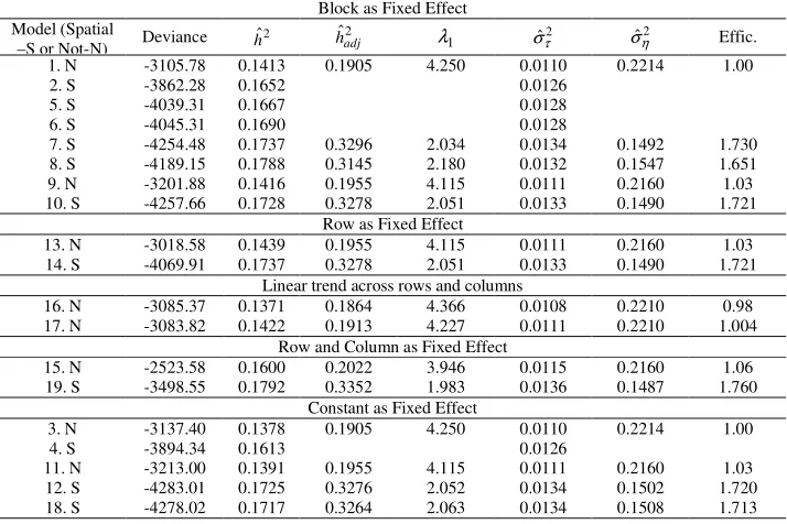
Table 1a - Summary of results concerning models 1 to 19 for trait leaf weight in the first year of harvest in trial 1. The estimates are: genetic variance among treatments (progenies) (_ˆ2

τ

σ ), non-correlated residual variance (σˆ_η2), narrow sense heritability (_hˆ2), fitted narrow sense heritability (hˆadj2 =(4σˆτ2)/(σˆτ2+σˆη2₎)

proportional only to the unaccounted error (η), shrinkage factor

( (ˆ2 3ˆ2)/(4ˆ2)

1 ση στ στ

λ= − ) of genetic effects in the mixed model equations and

efficiency (Effic.) of models over model1, in terms of hˆ_adj2 Block as Fixed Effect

Model (Spatial

–S or Not-N) Deviance hˆ2 hˆadj2 λ1 σˆτ2 σˆη2 Effic.

1. N -3105.78 0.1413 0.1905 4.250 0.0110 0.2214 1.00

2. S -3862.28 0.1652 0.0126

5. S -4039.31 0.1667 0.0128

6. S -4045.31 0.1690 0.0128

7. S -4254.48 0.1737 0.3296 2.034 0.0134 0.1492 1.730

8. S -4189.15 0.1788 0.3145 2.180 0.0132 0.1547 1.651

9. N -3201.88 0.1416 0.1955 4.115 0.0111 0.2160 1.03

10. S -4257.66 0.1728 0.3278 2.051 0.0133 0.1490 1.721

Row as Fixed Effect

13. N -3018.58 0.1439 0.1955 4.115 0.0111 0.2160 1.03

14. S -4069.91 0.1737 0.3278 2.051 0.0133 0.1490 1.721

Linear trend across rows and columns

16. N -3085.37 0.1371 0.1864 4.366 0.0108 0.2210 0.98

17. N -3083.82 0.1422 0.1913 4.227 0.0111 0.2210 1.004

Row and Column as Fixed Effect

15. N -2523.58 0.1600 0.2022 3.946 0.0115 0.2160 1.06

19. S -3498.55 0.1792 0.3352 1.983 0.0136 0.1487 1.760

Constant as Fixed Effect

3. N -3137.40 0.1378 0.1905 4.250 0.0110 0.2214 1.00

4. S -3894.34 0.1613 0.0126

11. N -3213.00 0.1391 0.1955 4.115 0.0111 0.2160 1.03

12. S -4283.01 0.1725 0.3276 2.052 0.0134 0.1502 1.720

18. S -4278.02 0.1717 0.3264 2.063 0.0134 0.1508 1.713

The deviance criterion is not adequate for comparing models with different fixed effects. So, efficiency in terms of the fitted heritability (proportional only to the unaccounted error) can be used for inference about the best models. The fitted narrow sense heritability estimates presented in the previous table refer to individual plant models rather then parent models.

The two traits (sequence measurements in consecutive years) presented approximately the same behaviour in terms of results across models. Among the non-spatial models, the row-column analyses (models 11, 13 and 15) performed better than the randomised block analyses (models 1 and 3). This can be explained by the local control in two directions provided by the row-column analysis and by the small block provided by rows since each original block was composed of six rows. Due to this last reason there was no need to fit blocks additionally to rows and columns (models 9, 10 and 17).

(12)

models with inclusion of η (models 7, 8, 10, 12, 14, 18 and 19) were always better than those without η (models 2, 4, 5 and 6) as judged by deviances of the models as well as selection efficiencies in terms of the fitted heritabilities or shrinkage factors for treatment effects in the mixed model equations (Tables 1a and 1b).

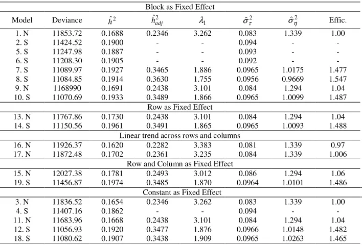
Table 1b - Summary of results concerning models 1 to 19 for trait leaf weight in the second year of harvest in trial 1. The estimates are: genetic variance among treatments (progenies) (_ˆ2

τ

σ ), non-correlated residual variance (σˆη2), narrow sense heritability (_hˆ2_{), fitted narrow sense heritability (}ˆ2 ₍₄_ˆ2₎_/(_ˆ2 _ˆ2₎

η τ τ σ σ

σ +

= adj

h )

proportional only to unaccounted error (η), shrinkage factor ( (ˆ2 3ˆ2)/(4ˆ2)

1 ση στ στ

λ= − )

of genetic effects in the mixed model equations and efficiency (Effic.) of models over model1, in terms of ˆ2

adj

h

Block as Fixed Effect

Model Deviance _hˆ2 ˆ2

adj

h λ1 σˆτ2 σˆη2 Effic.

1. N 11853.72 0.1688 0.2346 3.262 0.083 1.339 1.00

2. S 11424.52 0.1900 - - 0.094 - -

5. S 11247.98 0.1887 - - 0.093 - -

6. S 11208.30 0.1905 - - 0.092 - -

7. S 11089.97 0.1927 0.3465 1.886 0.0965 1.0175 1.477

8. S 11084.85 0.1914 0.3630 1.755 0.0956 0.9669 1.547

9. N 1168990 0.1691 0.2438 3.101 0.084 1.294 1.04

10. S 11070.69 0.1933 0.3489 1.866 0.0965 1.0099 1.487

Row as Fixed Effect

13. N 11767.86 0.1730 0.2438 3.101 0.084 1.294 1.04

14. S 11150.56 0.1961 0.3491 1.865 0.0965 1.0093 1.488

Linear trend across rows and columns

16. N 11926.37 0.1620 0.2282 3.383 0.081 1.339 0.97

17. N 11872.48 0.1702 0.2361 3.235 0.084 1.339 1.006

Row and Column as Fixed Effect

15. N 12027.38 0.1781 0.2493 3.012 0.086 1.294 1.06

19. S 11456.87 0.1974 0.3485 1.870 0.0964 1.0101 1.486

Constant as Fixed Effect

3. N 11836.52 0.1654 0.2346 3.262 0.083 1.339 1.00

4. S 11407.16 0.1862 - - 0.094 - -

11. N 11683.96 0.1668 0.2438 3.101 0.084 1.294 1.04

12. S 11056.93 0.1920 0.3477 1.876 0.0966 1.0148 1.482

18. S 11080.62 0.1907 0.3438 1.909 0.0965 1.0263 1.465

Comparing models 7, 12 and 18, which led to almost the same efficiency, can see that keeping the design features in the analysis was not necessary. The rate of recovering of design features by spatial analysis is enhanced when the independent error is fitted. A model without plot and design features was fitted for the two traits and provided almost the same efficiency as model 12, showing that sometimes simple spatial models can be used.

(13)

Little difference (in terms of fitted heritability), if any, was noted in fitting local control as fixed or random effects in the non-spatial models (model 1 against 3; 11 against 13 or 15) and spatial models (12 against 14 and 19), with a slight superiority for fitting row and column as fixed effects.

Overall, the best methods for the two traits were 12 and 14, both corresponding to a row-column analysis + a spatial (AR1 x AR1) + independent term error. For these best models, efficiency over the traditional randomised complete block analysis ranged from 1.48 to 1.76, i.e., 48% to 76% of superiority. Improved designs can be used to have high efficiency when assuming a spatial model such as model 12 (establishing the experiment according to model 12). In other words, appropriate systematic designs are needed when spatial patterns are present in the field. Spatial analysis has been shown to improve the precision and accuracy of treatment estimates, even with designs not optimised spatially. It is expected that designs with good general spatial properties will further increase the efficiency of treatments estimates. This would permit the fitting of only one spatial model to all trials as advocated by Kempton et al. (1994).

The autocorrelation coefficients for models without independent errors were approximately 0.21 and 0.29 for AR Column and 0.13 and 0.14 for AR Row, for the two traits, respectively. For models with independent errors, the autocorrelation coefficients were approximately 0.79 and 0.75 for AR Column and 0.50 and 0.52 for AR Row, for the two traits, respectively. These high autocorrelation coefficients obtained show that the AR process is modelling fertility gradient rather than competition. This is coherent with the spacing used (3 by 2 meters) and with crop management in which all the leaves are harvested each year. These features tend to prevent above ground competition between plants.

Models with splines were also tried, some extending the previous model 12 and others using only splines to account for spatial variation. Results are presented in Table 2.

It can be seen that the extended model 12 did not improve the fit through the inclusion of splines. The deviances of the extended models were higher as the spline variance component is constrained to be positive, but the efficiencies in terms of the fitted heritability were practically the same (Table 2).

The approach using splines in place of AR(1) x AR(1) process for modelling spatial variation was suggested by Kempton (1999) and used by Durban et al. (2001). In our data set, such approach showed to be very inefficient, being comparable only with the random row and column analysis (model 11).

Results concerning individual analysis of trial 2 of tea plants are presented in Table 3.

(14)

Table 2 - Results concerning some models for trait leaf weight in the first two years of harvest in trial 1. The estimates are: genetic variance among treatments (progenies) ( _ˆ2

τ

σ ), non-correlated residual variance (_ˆ2 η

σ ), fitted narrow sense heritability (hˆadj2 =(4σˆg2)/(σˆ2g+σˆη2)) proportional only to the unaccounted error (η) and efficiency (Effic.) of models over model 1, in terms of

h

ˆ

_adj2 . Spl(rc) means cubic splines applied on row and columns

Model Deviance ˆ2

adj

h _ˆ2

τ

σ _ˆ2

η

σ Eff.

Leaf weight 1 – Trial 1

1 -3105.78 0.1905 0.0110 0.2214 1.00

11 -2523.58 0.1955 0.0111 0.2160 1.03

Spl(rc) -3202.72 0.1961 0.0112 0.2173 1.03

12 -4283.01 0.3276 0.0134 0.1502 1.72

12 + Spl(rc) -4270.12 0.3302 0.0134 0.1489 1.73

Leaf weight 2 – Trial 1

1 11853.72 0.2346 0.0830 1.3390 1.00

11 11683.96 0.2438 0.0840 1.2940 1.04

Spl(rc) 11731.32 0.2464 0.0852 1.2979 1.05

12 11056.93 0.3477 0.0966 1.0148 1.48

12 + Spl(rc) 11070.08 0.3492 0.0965 1.0088 1.49

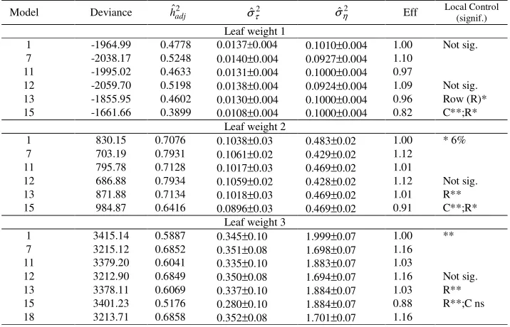
Table 3 - Results concerning some models for trait leaf weight in the first three years of harvest in trial 2. The estimates are: genetic variance among treatments (progenies) ( _ˆ2

τ

σ ), non-correlated residual variance (_ˆ2 η

σ ) and fitted narrow sense heritability (hˆadj2 =(4σˆg2)/(σˆ2g+σˆ_η2)) proportional only to unaccounted error (η)

and efficiency (Effic.) of models over model 1, in terms of _hˆ_adj2

Model Deviance hˆadj2 σˆτ2 σˆη2 Eff Local Control _(signif.)

Leaf weight 1

1 -1964.99 0.4778 0.0137±0.004 0.1010±0.004 1.00 Not sig.

7 -2038.17 0.5248 0.0140±0.004 0.0927±0.004 1.10 11 -1995.02 0.4633 0.0131±0.004 0.1000±0.004 0.97

12 -2059.70 0.5198 0.0138±0.004 0.0924±0.004 1.09 Not sig.

13 -1855.95 0.4602 0.0130±0.004 0.1000±0.004 0.96 Row (R)*

15 -1661.66 0.3899 0.0108±0.004 0.1000±0.004 0.82 C**;R*

Leaf weight 2

1 830.15 0.7076 0.1038±0.03 0.483±0.02 1.00 * 6%

7 703.19 0.7931 0.1061±0.02 0.429±0.02 1.12

11 795.78 0.7128 0.1017±0.03 0.469±0.02 1.01

12 686.88 0.7934 0.1059±0.02 0.428±0.02 1.12 Not sig.

13 871.88 0.7134 0.1018±0.03 0.469±0.02 1.01 R**

15 984.87 0.6416 0.0896±0.03 0.469±0.02 0.91 C**;R* Leaf weight 3

1 3415.14 0.5887 0.345±0.10 1.999±0.07 1.00 **

7 3215.12 0.6852 0.351±0.08 1.698±0.07 1.16

11 3379.20 0.6041 0.335±0.10 1.883±0.07 1.03

12 3212.90 0.6849 0.350±0.08 1.694±0.07 1.16 Not sig.

13 3378.11 0.6069 0.337±0.10 1.884±0.07 1.03 R**

15 3401.23 0.5176 0.280±0.10 1.884±0.07 0.88 R**;C ns

(15)

For this trial, column effects should not be fitted as fixed (model 15) as it is so small (size 30) and genetic information would be lost. With spatial analysis and inclusion of the independent error in the model, there was no need to include the design features in the model, even when the block effects were significant (trait 3). It can be seen from the deviance values that the model 7 and 18 were equivalent (Table 3). The auto-correlation coefficients were of the order of 0.80 and 0.90 between rows and columns, respectively, for the three traits (0.79 and 0.87; 0.79 and 0.87; 0.81 and 0.90, for traits 1, 2 and 3, respectively, according to the model 12).

3.2 Longitudinal non-spatial models for several measures on each trial

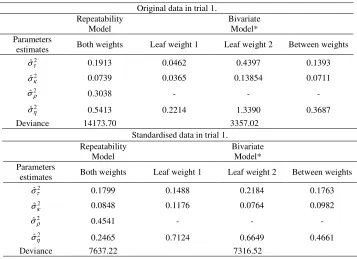
Results concerning repeatability and full unconstrained (bivariate in this case) models for the repeated measures in trial 1 are presented in Table 4. Block, measure and block x measure interaction effects were fitted as fixed.

Table 4 - Estimates of the variance parameters: genetic among treatments (progenies) ( _ˆ2

τ

σ ), among plots (_ˆ2 κ

σ ), permanent (_ˆ2 ρ

σ ) and residual (_ˆ2 η

σ ), using the repeatability and full unconstrained (bivariate) models

Original data in trial 1. Repeatability

Model Bivariate Model*

Parameters

estimates Both weights Leaf weight 1 Leaf weight 2 Between weights

2

ˆ_τ

σ 0.1913 0.0462 0.4397 0.1393

2

ˆ_κ

σ 0.0739 0.0365 0.13854 0.0711

2

ˆ_ρ

σ 0.3038 - - -

2

ˆ_η

σ 0.5413 0.2214 1.3390 0.3687

Deviance 14173.70 3357.02

Standardised data in trial 1. Repeatability

Model Bivariate Model*

Parameters

estimates Both weights Leaf weight 1 Leaf weight 2 Between weights

2

ˆ_τ

σ 0.1799 0.1488 0.2184 0.1763

2

ˆ_κ

σ 0.0848 0.1176 0.0764 0.0982

2

ˆ_ρ

σ 0.4541 - - -

2

ˆ_η

σ 0.2465 0.7124 0.6649 0.4661

Deviance 7637.22 7316.52

(16)

show that the bivariate model is much better than the repeatability model. This justifies the preference for the bivariate model.

With standardised data (divided by the phenotypic standard deviation from individual analysis for each measure), the associated repeatability coefficient was 0.75, which is higher than the previous one. Standardisation led to an increased permanent variance estimate, while the others (except by the independent error) variance components were kept approximately constant (in comparison to the data in original scale) by the repeatability model. The genetic correlation coefficient between the two measures in the bivariate analysis was 0.98, which was the same as in the previous analysis. However, it can be seen that the heterogeneity of variance was reduced after standardisation. The deviance values show that the repeatability and bivariate models became closer after standardisation.

Nevertheless, the AIC values were 7334.52 and 7645.22 for the bivariate and repeatability models. This shows that the bivariate model, although less parsimonious, is still better than the repeatability model. So, in practice, the bivariate model should be used for selection. In case the repeatability model is chosen, the data should at least be standardised. The use of the bivariate model for selection implies giving weight to genetic values predicted for the two measures. These weights should be 0.5, if the two ages have equal importance. If the last measure provides a better representation of a mature trait, higher weight should be given to this measure. Nonetheless, the high genetic correlation may suggest that the weights should be 0.5 for each measure.

Estimates for the full (multivariate) model with original data in trial 2 are presented in Table 5. Block, measure and block x measure interaction effects were fitted as fixed. Table 5 - Estimates of the variance and covariance parameters for the full (multivariate)

model with original data in trial 2 concerning three repeated measures. Number of parameters equal to 18

Treatment (genetic) Plot Residual

Covar.\Variance\Correl. Covar.\Variance\Correl. Covar.\Variance\Correl. 0.0134 0.9239 0.9984 0.0248 0.8638 0.7095 0.1011 0.6766 0.6128 0.0342 0.1020 0.9211 0.0422 0.0964 0.9123 0.1495 0.4827 0.7686 0.0673 0.1711 0.3380 0.0817 0.2072 0.5352 0.2755 0.7551 1.9990

Deviance = -787.172

The deviance value (Table 5) reveals that the full multivariate model is far more suitable for the original data than the repeatability model (deviance 5070.64, results not shown). Such model gave high values for the genetic correlations between pairs of measures. The correlations were all within the parameter space but the model had to be constrained to achieve this. Without constraining the G matrix to be positive definite, correlations higher than 1 and negative variance components were obtained. In the constrained model, the G matrix is bent and this process involves shrinking the variances towards their mean. The unconstrained analysis is less biased because bias is introduced when constraining the solution to the parameter space. Convergence was more difficult as the number of measures increased. So, more suitable models needed to be searched.

(17)

Table 6 - Estimates of the variance and covariance parameters for the character process model, called first order autoregressive with heterogeneous variance (ARH) applied to original data in trial 2, concerning three repeated measures. Number of parameters equal to 16

Deviance = -782.94

The ARH and multivariate models presented almost the same deviance and the AIC values were -750.94 and -751.17, respectively, which are basically the same –751. So, the two models are equivalent by the parsimony criterion. However, ARH presented easy convergence without constraining the G matrix to be positive definite, fitted a small (two less than the full multivariate model) number of parameters and gave correlations within the parameter space. Besides, it gave a more realistic correlation between the most distant measures 1 and 3. The ARH model is then much preferred. Such model assumes stationarity and same correlation in all intervals of same lag.

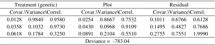
An other model evaluated was the structured ante-dependence model (SAD), which also has parsimony and does not assume stationarity. Results are presented in Table 7. Table 7 - Estimates of the variance and covariance parameters for the structured

ante-dependence model (SAD) with original data in trial 2, concerning three repeated measures. Number of parameters equal to 17

Deviance = -783.04

The SAD and ARH models presented basically the same deviance (-783) and are then equivalent by this criterion. Nonetheless, the SAD model fitted one parameter more than the ARH model and is not preferred, in terms of parsimony by the AIC rule. The results for plot and residual effects were exactly the same by the two models. The genetic components were slightly different but are both coherent in terms of the magnitude of the correlation coefficients, i.e., smaller for lag 1-3. This was not seen in the full multivariate model. Both models could be used efficiently in practice. The SAD model allows for different correlation for lags of same size.

(18)

Table 8 - Estimates of the correlation parameters for the structured ante-dependence model (SAD) and character process (ARH) for modelling both the treatment and plot effects. An original data set in trial 2 (three repeated measures) was used. Number of parameters equal to 16 and 14 for SAD and ARH, respectively.

ARH\SAD ARH\SAD ARH\SAD

- 0.990 0.968 - 0.851 0.769 - 0.6766 0.6128

0.982 - 0.977 0.882 - 0.903 0.6766 - 0.7686

0.964 0.982 - 0.778 0.882 - 0.6128 0.7686 -

Deviance ARH\SAD = -780.76\-782.20

The results show that the plot effect can be perfectly modelled by the ARH or SAD process. The deviance values were close to the previous one where the plot effect was modelled in a full multivariate fashion. The AIC values here were –752.76 and –750.20 for ARH and SAD, respectively, which are close to values –751 and –749 for ARH and SAD, respectively, obtained with the two models but with multivariate plot effect. Comparing these four AIC values, the choice is for the ARH model for both treatments and plot effects (AIC –752.76).

The modelling of the residual term by the ARH was also evaluated. The resulting deviance for modelling the three effects simultaneously as an ARH process gave a deviance of only –677.46. Also the residual correlations obtained were very different than the previous ones. Then, the residual should be modelled in a full multivariate way.

Other approaches were also evaluated. The banded correlation or Toeplitz model converged with a deviance of –794.28. Nevertheless, it gave a genetic correlation higher than one, and only the correlation was supposed to be the small one. This model assumes equal correlation for lags of same size as does the ARH model, but the elements of the several diagonals are different and not a function of the correlation for lag 1.

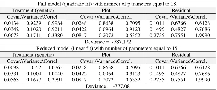
Random regression models were also tried and results are presented in Table 9 for the full and reduced models.

Table 9 - Estimates of the variance and covariance parameters for the random regression model with original data in trial 2 concerning three repeated measures

Full model (quadratic fit) with number of parameters equal to 18.

Deviance = -787.172

Reduced model (linear fit) with number of parameters equal to 15.

(19)

Results were identical to those (which were not suitable) from the full multivariate analysis as expected for the full fitting of the random regression model, i.e., for fitting a quadratic polynomial. In a search for parsimony a reduced fit was tried. The deviance (-777) of the model is higher than that (-783) obtained from the ARH and SAD models for treatment effects (Tables 8 and 9). The AIC value is –747, which is higher than that obtained for the ARH (-751) and SAD (-749) models. So, the reduced random regression model is not a choice. Also, this model showed a poor reconstruction of the G matrix for treatment effects leading all correlations to be higher than 1 (Table 9). These results are in accordance with Apiolaza et al. (2000), who found that random regression models were often inappropriate.

The fit of smoothing cubic splines was also tried. The deviance obtained was only – 748.33, which was the worst between the parsimonious models tried. This result was expected as function of the small number of ages available for fitting. In conclusion, the best approaches for trial 2 were the ARH and SAD models for treatment and plot effects. These models should be extended and used in conjunction with the spatial models for the residuals.

3.3 Longitudinal spatial models for repeated measures on each trial

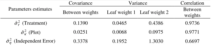
Results concerning the multivariate spatial model for trial 1 are presented in Table 10.

Table 10 - Estimates of the variance parameters: genetic variance among treatments (progenies) (

σ

ˆ

_τ2), among plots (

σ

ˆ

_κ2), residual (

σ

ˆ

_η2) and respective covariance and correlation by the full multivariate spatial model for leaf weight in trial 1

Covariance Variance Correlation

Parameters estimates _{Between weights} _{Leaf weight 1 Leaf weight 2} Between weights

2

ˆ_τ

σ (Treatment) 0.1390 0.0465 0.4386 0.9736

2

ˆ_κ

σ (Plot) 0.0251 0.0068 0.0975 0.9771

2

ˆ_η

σ (Independent Error) 0.3378 0.1952 1.3030 0.6697

Deviance = 2764.12

(20)

For trial 2, the superior approaches for analysing the repeated measures were extended by incorporating spatially correlated residuals. Three models were tried: ARH for treatments, ARH for treatments and plots and SAD for treatments and plots. The deviance values obtained were not lower than that obtained with the best non-spatial models and, the autocorrelation parameters approached 1, revealing that there is no need for spatial analysis for this multivariate data. This was expected as the efficiency of spatial analysis for the univariate case in this experiment was low as a function of the low environmental variability in the trial. In the multivariate case for the repeated measures, the amount of information about one individual increase and the model is automatically improved making it more difficult to add important information from the spatial analysis. Besides, the autocorrelation estimates approached 1, revealing that the estimated correlated error was of small magnitude.

4

Final conclusions

For longitudinal data or repeated measured traits (sequence measurements in consecutive years) in perennial crops, which exhibit considerable variance heterogeneity between traits and high correlation between measures, the repeatability and the full unconstrained models are not adequate, revealing a need for new modelling. In general, the best approaches involved the modelling of treatment effects by ante-dependence (SAD) or auto-regressive models with heterogeneous variance (ARH). When spatial effects are important, a combination of the first-order spatial auto-regressive approach for modelling errors and a multivariate (including simpler options such as SAD and ARH) approach for modelling treatments effects should be used.

RESENDE, M. D. V. de; THOMPSON, R.; WELHAM, S. Análise estatística espacial multivariada de dados longitudinais em culturas perenes. Rev. Mat. Est., São Paulo, v. 24, n.1, p.147-169, 2006.

(21)

erro (AR1 x AR1); as diferentes medidas repetidas apresentaram aproximadamente o mesmo comportamento em termos de resultados através dos diferentes modelos; os modelos de repetibilidade e multivariado não foram totalmente adequados para a análise de medidas repetidas, as quais exibiram considerável heterogeneidade de variâncias, revelando a necessidade da adoção de novas modelagens. Em geral, as melhores abordagens envolveram a modelagem dos efeitos de tratamentos por modelos autoregressivos (ARH) e de ante-dependência (SAD) com variâncias heterogêneas. Quando os efeitos espaciais são importantes, a combinação de modelos autoregressivos para os resíduos e modelos SAD ou ARH para os efeitos de tratamentos, deve ser usada na análise de medidas repetidas em plantas perenes.

PALAVRAS-CHAVE: Medidas repetidas; tendência ambiental; modelos mistos; reml; blup; modelos autoregressivos; modelos ante-dependência.

5

References

APIOLAZA, L. A.; GILMOUR, A. R.; GARRICK, D. J. Variance modelling of longitudinal height data from a Pinus radiata progeny test. Can. J. For. Res., Ottawa, v. 30, p. 645-654, 2000.

ATKINSON, A.C. The use of residuals as a concomitant variable. Biometrika, London, v.56, p.33-41, 1969.

BANERJEE, S.; CARLIN, B.; GELFAND, A. Hierarchical modelling and analysis for spatial data. London: Chapman & Hall, 2003. 488p.

BARTLETT, M.S. The approximate recovery of information from replicated field experiments with large blocks. J. Agric. Sci., Cambridge, v.28, p.418-427, 1938.

BARTLETT, M.S. Nearest neighbour models in the analysis of field experiments. J. R. Stat. Soc. Ser. B., London, v. 40, p.147-174, 1978.

BESAG, J.; KEMPTON, R.A. Statistical analysis of field experiments using neighbouring plots. Biometrics, Washington, v. 42, p. 231 – 251, 1986.

COOPER, D.M.; THOMPSON, R. A note on the estimation of the parameters of the autoregressive-moving average process. Biometrika, London, v. 64, p. 625-628, 1977. CRESSIE, N.A.C. Statistics for spatial data analysis. New York: John Wiley & Sons, 1993. 900p.

CULLIS, B. R. et al. Spatial analysis of multi-environment early generation variety trials.

Biometrics, Washington, v. 54, p.1-18, 1998.

CULLIS, B.R.; GLEESON, A.C. Spatial analysis of field experiments-an extension at two dimensions. Biometrics, Washington, v.47, p.1449-1460, 1991.

DURBAN, M.; CURRIE, I.; KEMPTON, R. Adjusting for fertility and competition in variety trials. J. Agric. Sci., Cambridge, v.136, p.129-149, 2001.

FISHER, R. A. Statistical methods for research workers. 1. ed. London: Oliver and Boyd, 1925. 314 p.

(22)

GILMOUR, A.R. et al. (Co)variance structures for linear models in the analysis of plant

improvement data. In: COMPSTAT98, 1998. Proceedings … Heidelberg: Physica -

Verlag, 1998. p.53-64.

GILMOUR, A.R. Post blocking gone too far! Recovery of information and spatial analysis in field experiments. Biometrics, Washington, v. 56, p.944 – 946, 2000.

GILMOUR, A. R.; THOMPSON, R. Modelling variance parameters in ASREML for repeated measures. In: WORLD CONGRESS ON GENETIC APPLIED TO

LIVESTOCK PRODUCTION, 6., 1998, Armidale. Proceedings… Armidale: AGBU /

University of New England, 1998. v. 27, p. 453-454.

GILMOUR, A. R.; THOMPSON, R.; CULLIS, B. R. Average information REML: an efficient algorithm for parameter estimation in linear mixed models. Biometrics, Washington, v. 51, p.1440-1450, 1995.

GILMOUR, A. R. et al. ASReml reference manual. Release 1.0, 2nd. ed. Harpenden: Biomathematics and Statistics Department - Rothamsted Research, 2002. 187 p.

GLEESON, A.C. Spatial analysis. In: KEMPTON, R.A; FOX, P.N. Statistical methods for plant variety evaluation. London: Chapman & Hall, 1997. Chapter 5, p.68-85.

GLEESON, A.C.; CULLIS, B.R. Residual maximum likelihood (REML) estimation of a neighbour model for field experiments. Biometrics, Washington, v.43, p.277-288, 1987. GREEN, P.J.; JENNISON, C.; SEHEULT, A. Analysis of field experiments by least square smoothing. J.R. Statist. Soc. Ser. B., London, v. 47, n.2, p.299-315, 1985.

GREEN, P. J.; SILVERMAN, B. W. Nonparametric regression and generalized linear models. London: Chapman & Hall. 1994. 182 p.

GRONDONA, M.O.; CRESSIE, N. Using spatial considerations in the analysis of experiments. Technometrics, Washington, v. 33, p.381–392, 1991.

GRONDONA, M. O. et al. Analysis of variety yield trials using two-dimensional

separable ARIMA processes. Biometrics, Washington, v.52, p.763-770, 1996.

HENDERSON, C.R. Aplications of linear models in animal breeding. Guelph: University

of Guelph, 1984. 462p.

JAFFREZIC, F.; PLETCHER, S.D. Statistical models for estimating the genetic basis of repeated measures and other function valued traits. Genetics, Bethesda, v. 156, p. 913-922, 2000.

JAFFREZIC, F. et al. Statistical models for the genetic analysis of longitudinal data. In: WORLD CONGRESS OF GENETICS APPLIED TO LIVESTOCK PRODUCTION, 7. Montpellier. Communication n. 16-08. Montpellier: INRA, 2002. 4p, 2002.

JOHNSON, D. L.; THOMPSON, R. Restricted maximum likelihood estimation of variance components for univariate animal models using sparse matrix techniques and average information. J. Dairy Sci., Savoy, v.78, p. 449-456, 1995.

(23)

KEMPTON, R. A. Discussion on The analyses of designed experiments and longitudinal data using smootthing splines. (By VERBYLA, A.P; CULLIS, B.R.; KENWARD, M.G.; WELHAM, S.J.) J. R. Stat. Soc., Ser. C., London, v.48, p.300-301, 1999.

KIRKPATRICK, M.; HILL, W. G.; THOMPSON, R. Estimating the covariance structure of traits during growth and ageing, illustrated with lactations in dairy cattle. Genet. Res., London, v. 64, p.57-69, 1994.

MARTIN, R.J. The use of time-series models and methods in the analysis of agricultural field trials. Commun. Stat. Theory Methods, New York, v.19, n.1, p.55-81, 1990.

MEYER, K.; HILL, W. G. Estimation of genetic and phenotypic covariance functions for longitudinal or repeated records by restricted maximum likelihood. Livest. Prod. Sci., Amsterdan, v. 47, p.185-200, 1997.

NUNEZ-ANTON V.; ZIMMERMANN, D.L. Modelling non-stationary longitudinal data.

Biometrics, Washington, v.56, p.699-705, 2000.

PAPADAKIS, J. Method statistique pour des experiences sur champ. Bull.Inst.

d’Amelioration Plantes Salonique. Thessalonique, v.23, 1937.

PAPADAKIS, J. Agricultural research: principles, methodology, suggestions. Buenos Aires: Edicion Argentina, 1970.

PAPADAKIS, J. Advances in the analysis of field experiments. Commun. Acad. Athenes,

Athenas, v.59, p.326-342, 1984.

PATTERSON, H. D.; THOMPSON, R. Recovery of inter-block information when block sizes are unequal. Biometrika, London, v.58, p.545-554, 1971.

PLETCHER, S.D.; GEYER, C.J. The genetic analysis of age-dependent traits: modelling a character process. Genetics, Bethesda, v.153, p.825-833, 1999.

QIAO,C. G. et al. Evaluation of experimental designs and spatial analysis in wheat breeding trials. Theor. Appl. Genet., Berlin, v. 100, p.9-16, 2000.

SEARLE, S.R.; CASELLA, G.; Mc CULLOCH, C.E. Variance Components. New York:

John Wiley, 1992. 528p.

SMITH, A.; CULLIS, B.R.; THOMPSON, R. Analysing variety by environment data using multiplicative mixed models and adjustment for spatial field trend. Biometrics, Washington, v. 57, p. 1138-1147, 2001.

STEEL, R.G.D.; TORRIE, J.H. Principles and procedures of statistics. 2th. ed. New York: Mac Graw-Hill, 1980. 633p.

STRINGER, J.K.; CULLIS, B.R. Application of spatial analysis techniques to adjust for fertility trends and identify interplot competition in early stage sugarcane selection trials.

Aust. J. Agric. Res., Collingwood, v.53, n.8, p.911-918, 2002.

THOMPSON, R.; WELHAM, S. J. REML analysis of mixed models. In: PAYNE et al. (Ed). GenStat 6 release 6.1. The guide to GenStat, Statistics. Harpenden: Rothamsted Research, 2003. p.469-560.

(24)

Rev. Mat. Estat., São Paulo, v.24, n.1, p.147-169, 2006 169 VERBYLA, A.P; CULLIS, B.R.; KENWARD, M.G.; WELHAM, S.J. The analyses of designed experiments and longitudinal data using smootthing splines. J. R. Stat. Soc., Ser. C., London, v.48, p.269-311, 1999.

WHITE, I. M. S.; THOMPSON, R.; BROTHERSTONE, S. Genetic and environmental smoothing of lactation curves with cubic splines. J. Dairy Sci., Savoy, v.82, p.632-638, 1999.

WILKINSON, G.N.; ECKERT, S.R.; HANCOCK, T.W.; MAYO, O. Nearest neighbor (NN) analysis of field experiments. J. R. Stat. Soc. Ser. B., London, v.45, p.151-211, 1983.

WILLIAMS, E.R. A neighbor model for field experiments. Biometrika, London, v.73, p.279-287, 1986.

ZIMMERMAN, D.I.; HARVILLE, D.A. A random field approach to the analysis of field-plot experiments and other spatial experiments. Biometrics, Washington, v.47, p.223-239, 1991.