An exact test to detect geographic aggregations of events

M E T H O D O L O G Y

Open Access

An exact test to detect geographic aggregations

of events

Rhonda J Rosychuk

1,2*

, Jason L Stuber

3

Abstract

Background:Traditional approaches to statistical disease cluster detection focus on the identification of geographic areas with high numbers of incident or prevalent cases of disease. Events related to disease may be more appropriate for analysis than disease cases in some contexts. Multiple events related to disease may be possible for each disease case and the repeated nature of events needs to be incorporated in cluster detection tests.

Results:We provide a new approach for the detection of aggregations of events by testing individual

administrative areas that may be combined with their nearest neighbours. This approach is based on the exact probabilities for the numbers of events in a tested geographic area. The test is analogous to the cluster detection test given by Besag and Newell and does not require the distributional assumptions of a similar test proposed by Rosychuk et al. Our method incorporates diverse population sizes and population distributions that can differ by important strata. Monte Carlo simulations help assess the overall number of clusters identified. The population and events for each area as well as a nearest neighbour spatial relationship are required. We also provide an alternative test applicable to situations when only the aggregate number of events, and not the number of events per individual, are known. The methodology is illustrated on administrative data of presentations to emergency departments.

Conclusions:We provide a new method for the detection of aggregations of events that does not rely on distributional assumptions and performs well.

Background

In disease surveillance, statistical methods can be used to identify geographical areas that have statistically higher numbers of cases of disease than expected by chance. These geographical areas with aggregations of disease are called clusters. In some situations, the dis-ease incidence or prevalence may not be the most or only relevant feature for analysis, and the analysis of events related to diseased individuals may be more appropriate. For the delivery of health services through emergency departments (EDs), the number of presenta-tions to EDs can be more relevant than the number of distinct individuals seen in the ED. If there are many individuals that have multiple presentations, analysis based solely on the number of individuals, and not the number of presentations, will only be able to identify

clusters with excess numbers of individuals and not clusters with excess presentations. Ignoring presenta-tions prevents identification of clusters where more pre-sentations, but not necessarily more individuals, are occurring than expected by chance. Surveillance of pre-sentations to EDs can identify geographic areas with high presentations where access to other health care providers is limited and statistical detection of these areas necessitates incorporating repeated presentations by individuals.

There are several different tests for the identification of clusters of diseased individuals (cases) in geographic areas (see [1,2] for overviews). The geographic areas are generally administrative regions for which case and population counts are available. Besag and Newell [3] used the terms general and focused to distinguish between tests that identify clusters in a geographic region and those that identify clusters around specific geographic locations, such as hazardous waste sites. For * Correspondence: [email protected]

1_{Department of Pediatrics, 11402 University Avenue NW, Edmonton, Alberta,}

Canada

both types of tests, the methods generally either exam-ine areas with similar population size and compare the number of cases or examine areas with similar numbers of cases and compare the population sizes. Some meth-ods can detect the location of clusters while others can identify areas with the tendency to cluster.

We focus on methods that can accommodate geo-graphic areas with different population sizes. One explora-tory method has been proposed by Openshaw et al. [4] and requires the user to specify a threshold. Their geo-graphic analysis machine constructs overlapping circles and displays the circles with proportions of cases exceed-ing the threshold. The Turnbull et al. [5] method also uses overlapping circles but these circles require a user-speci-fied population size. The maximum number of cases in each of the circles is determined and a Monte Carlo test assesses if the observed proportion is higher than expected. Kulldorff and Nagarwalla [6] generalize this approach and seek to identify a clustered circle, where the individuals inside the circle have greater risk than the indi-viduals outside the circle, using a likelihood ratio test. Duczmal and Assunção [7] propose a similar approach that uses connected subgraphs to identify the cluster. Tango [8] takes a different strategy by using area propor-tions of cases and a measure of closeness. A chi-square test compares observed and expected proportions to detect clusters. Besag and Newell [3] look at similar num-bers of cases and combine nearby areas to observe a user-specified number of cases. The population sizes of these areas with similar cases are then compared. More recently, Rosychuk et al. [9] have provided a similar method for events rather than cases by using a compound Poisson dis-tribution and compared the two approaches [10].

Herein, we provide an approach to identify geographic areas with aggregations of events. These aggregations are called event clusters, or simply clusters when the distinction between aggregations of events and cases is clear. Our approach is analogous to the cluster detection test proposed by Besag and Newell [3] and does not require distributional assumptions, like the Rosychuk et al. [9] test. The approach is instead based on exact probabilities for the numbers of events in a tested geo-graphic area. The method incorporates diverse popula-tion sizes and populapopula-tion distribupopula-tions that can differ by important strata. This method requires the number of events per case is known. In addition, we provide an approach that can be used when the total number of events are known for the cases in a geographical area, but not the number of events per case. We describe the methodology and compare the methods using adminis-trative data on emergency department (ED) presenta-tions for self-inflicted injuries. We provide a simulation study that examines the false detection of clusters and conclude our discussion.

Results

We consider a geographic region divided into Icells where the population in celliis denoted byn_i,i= 1,...,I.

The total population is labeled n n_i

i I

=

∑

₌₁ . The

dis-tances between cell centroids are calculated for each pair of cells. For each cell, the remaining cells are ordered based on increasing pairwise distances to determine the nearest neighbours. Specifically, we leti1be the cell that is closest to celli,i2be the cell that is next closest to cell i, and so on. For convenience, we havei0=i.

We first describe the Besag and Newell [3] approach for cases using a hypergeometric distribution. We pro-vide our new exact method for events and review the compound Poisson approach developed by Rosychuk et al. [9]. We also describe the inclusion of strata vari-ables and the choice of event cluster size.

Hypergeometric approach for cases

The Besag and Newell [3] method requires the number of cases and population in each cell. For each cell i, let Cibe the random variable denoting the number of cases

in the cell and letci be the observed value. Further, let

C C_i

i I

=

∑

₌₁ and c c_i

i I

=

∑

₌₁ be the random variable

and the observed value of the total number of cases in the entire region, respectively. In practical applications for a rare disease, ci ≪ni and generally c≪ ni, for i=

1,...,I.

Each celliis tested separately and the test is based on combining nearest neighbours to obtain a minimum pre-specified number of cases, called the cluster size. For celli, suppose that the cluster size isk. The test sta-tistic, L_i, is the smallest number of nearest neighbours that must be combined withito have at leastkcases,

L_i q k C_i

a q a = ⎧⎨⎪ ≤ ⎩⎪ ⎫ ⎬ ⎪ ⎭⎪ =

∑

min such that .

0

Smaller observed values of Liare indicative of higher

numbers of cases in the vicinity of the tested cell. Under a null hypotheses that all individuals are equally likely to be a case independent of other cases and geographic location, Besag and Newell [3] use a Poisson distribution as an approximation to the hyper-geometric probability. Using the exact hyperhyper-geometric formulation, the probability that there are exactly xcases in a sample ofmpopulation is

If we denote the population of the combined cells as ni: _a nia



=

∑

₌₀ , then the significance level for the

tested cell becomes

pr(Li ) H x n( , i: ). x k ≤ = − = −

∑

 1 _

0 1

(2)

We will refer to this testing approach as the hyper-geometric case (HC) analysis in further discussions.

As each cell is tested separately and multiple testing is an issue, Besag and Newell [3] suggest Monte Carlo simulations to help assess the significance of overall clustering. Let R_a denote the number of cells that are significant at significance levela. For each simulation,

the c cases are randomly distributed to the I cells

according to the proportion of population in each cell (i.e., cases are distributed to cell ibased on probability ni/n). The testing is conducted and the number of

sig-nificant cells for each simulation is recorded. The overall assessment of statistical significance is obtained as the proportion of simulations that are at least as extreme as the observed Ra from the actual data set. We refer to

this overall assessment as a p-value for overall

clustering.

The proposed approaches for events

Our proposed method builds on the principles of the HC method and the approach of Rosychuk et al. [9] that concentrates on the number of disease-related events rather than the number of diseased individuals. As before, C_idenotes the random variable correspond-ing to the number of cases in cell i. LetV_i and v_i be the random variable and observed value of the number of events in cell i, respectively. The total number of cases (i.e., individuals with at least one event)

and events for the region are denoted by C C_i

i I =

∑

₌₁

and V V_i

i I

=

∑

₌₁ with observed values c c_i

i I

=

∑

₌₁ and

v v_i

i I

=

∑

₌₁ , respectively. In most applications, c_i <v_i≪ ni and c <v≪ ni for i = 1, ..., I, but such restrictions

are not required.

Each cell is tested separately as for the cases approach described above. The cluster size, now termed event cluster size, is the number of events rather than the number of cases used in the test. Let k* be the event cluster size for cell i. The test statistic is the smallest number of nearest neighbours that must be combined with cellito have at least k*events,

Li q k Vi

a q

a *

min * .

= ⎧_⎨⎪ ≤ ⎩⎪ ⎫ ⎬ ⎪ ⎭⎪ =

∑

such that 0 (3)

Smaller observed values of L*_i are indicative of higher numbers of events in the vicinity of the tested cell.

The use of events requires changes to the null hypoth-esis and the exact probability. The null hypothhypoth-esis is that every individual is equally likely to have events, independent of other individuals and geographic loca-tion. The hypergeometric probability is no longer appro-priate if there is more than one event per case. If the number of events per case is known, then a multiple hypergeometric approach can be used as described below. If the number of events per case is unknown but the total number of cases and events are known, then a counting approach which employs occupancy numbers can be used.

Known number of events per case

LetCiybe the random variable denoting the number of

cases in cell i that have exactly y events and let ciy

denote its observed value. Suppose that the maximum number of events any subject has isY, 1≤ Y. The total

number of cases in celliis C_i C_iy

y Y

=

∑

₌₁ and the total

number of cases in the entire study region with exactly

y events is C _y C_iy

i I

• =

∑

₌1 . Further, the total number of

cases is C C_i C

i I

y y Y

=

∑

₌₁ =

∑

₌₁ • For each cell i,

V_i yC_iy

y Y

=

∑

₌₁ is the number of events in the cell. The probability of the number of events observed in a geographic area is based on a multiple hypergeometric distribution, since individuals with the same number of events can be thought of as classes and the subjects are sampled without replacement from these classes. The

probability of observing x events among a sample of

mindividuals is

M x m

C r C r C Y rY n C

m r r _rY

( , )= • ⎛ ⎝ ⎜ ⎞ ⎠ ⎟⎛ • ⎝ ⎜ ⎞ ⎠ ⎟ ⎛ • ⎝ ⎜ ⎞ ⎠ ⎟⎛ _{− −}− ₋ ⎝ ⎜ 1 1 2

2 1 2

  ⎞⎞ ⎠ ⎟ ⎛ ⎝ ⎜ ⎞ ⎠ ⎟

∑

n m  , (4)

where {r_y} are non-negative integers from the set ,  = {(r1, ...,rY) such that x _y yry

Y

=

∑

₌₁ andry≤C•y,

y= 1, ..., Y} Note that if the maximum number of events per subject is one (Y = 1), then (4) simplifies to the hypergeometric distribution in (1). The significance level for the tested cellibecomes

pr( * ) ( , _: ),

*

L_i M x n_i

x k ≤ = − = −

∑

 1 _

0 1

(5)

In practical application, the random variables repre-senting events are replaced by the corresponding observed values and the expected number of events, ni:ℓv/n, is helpful in describing the results. Simulated

data sets are created analogously as described for the Besag and Newell approach for cases and a p-value for overall clustering is determined. We used a C++ pro-gram for numerical results and M (x, n_i:ℓ) is quite easily obtained by convoluting binomial coefficients and storing the intermediate quantities. The terms

n C

m r r r_Y

− − − − ⎛ ⎝ ⎜ ⎞ ⎠ ⎟

1 2

and n m ⎛ ⎝ ⎜ ⎞ ⎠

⎟ are common to each

combination of (r1, ..., rY), and thus can be

pre-computed and simplified for better numerical stability by using logarithms.

Our new approach is similar to the test provided by Rosychuk et al. [9]. The difference in approaches is the way in which the key probabilities are calculated. In that work [9], instead of the probability in (4), prob-abilities from a compound Poisson distribution are used. Specifically, P (x, n_i:ℓ) replaces M (x, n_i:ℓ) in (5) and is defined by

P_{( ,}n_{i )} e n C ni :

/

:

0 _ = −  ₍₆₎

P x n ni C

xn yQ y P x y n

x i i y x ( , _:)= : ( ) ( − , _:), ≥ =

∑

₁ 1 (7)

where Q(y) is the probability that a case has exactly y events. Those authors take Q(y) to be the observed frequency c•y/cand with this choice, the expected

num-ber of events becomes ni:ℓ (c/n) (v/c) = ni:ℓ v/n. This

approach, referred to as the compound Poisson event (CPE), assumes that a compound Poisson distribution is appropriate and relies on estimates of the Q(y) that may not be very precise. Both methods have the same expected number of events but these events come from distinct distributions. As in the HC approach for cases, Monte Carlo simulations can be used to help assess overall clustering.

Aggregate number of events known only

In some situations, the total number of events, v_i and

v, and cases may be known but the exact number of

events per case (e.g., ciy, c•y) may not be known. Here,

the relevant probability can be determined using a counting approach employing occupancy numbers (see [11] p. 38).

The number of ways that Vevents can be distributed

among thenindividuals is n V

V − + ⎛ ⎝ ⎜ ⎞ ⎠ ⎟ 1

. From a sample

population of size m, m x

x − + ⎛ ⎝ ⎜ ⎞ ⎠ ⎟ 1

is the number of

ways thatxevents can be distributed among them

indi-viduals and n m V x

V x − − + − − ⎛ ⎝ ⎜ ⎞ ⎠ ⎟ 1

is the number of ways

to distribute the remaining V - x events among the

remaining n - m individuals. Putting these counts

together, the probability of observingxevents among a sample ofmindividuals is

G

m x

x

n m V x

V x n V V x m ( , ) = . − + ⎛ ⎝ ⎜ ⎞ ⎠ ⎟⎛ − − + −₋ ⎝ ⎜ ⎞ ⎠ ⎟ − + ⎛ ⎝ ⎜ ⎞ ⎠ ⎟ 1 1 1 (8)

The significance level for the tested cell becomes

pr( * ) ( , _: ),

*

L_i G x n_i

x k ≤ = − = −

∑

 1 _

0 1

(9)

and we refer to this approach as the aggregate event (AE) analysis. As in the EE approach, random variables are replaced by the corresponding observed values and simulation is used to assess overall significance.

A key difference with this new aggregate event method and the EE and CPE methods is that the latter two methods link the events to cases. The AE approach uses only aggregate events, assumes that events are indistinguishable, and does not include information on the number of cases or the chance that a particular number of events are observed from one subject. Hence a loss of information occurs with the use of the AE approach, however if the information available does not include the number of events per case then the EE and CPE methods are not applicable and the AE method permits analysis.

Stratification

Cells can have population distributions that differ on key characteristics such as gender and age. These strata can be added to the test to adjust for differing popula-tion distribupopula-tions. Suppose there areSstrata. The popu-lation in cell i and stratum s is n_is, s = 1,..., S, and

relevant aggregate populations become n _s n_is

i I

and n _s nis S i I

=

∑

₌₁

∑

₌₁ . For stratum s, let C_iys be the random variable denoting the number of cases in cell i that have exactlyy events. The total number of cases in the entire study region in stratumswith exactlyy events

is C _ys C_iys

i I

• =

∑

₌1 . Similarly, Vis is the number of

events in cell iand stratumsand the number of events

in celliis V_i V_is yC

s S iys y Y s S

=

∑

₌₁ =

∑

₌₁

∑

₌₁ .

The test statistic in (3) also applies when strata are added. The relevant probability is based on (4), but has to be modified to include the different strata and the multiple ways that the events may be distributed amongst the strata. The probability of observing

x events among a sample ofm =m1 ++mS

indivi-duals is

M x m m

C _s r s C _s r s C Ys rYs

n s C

S ( , ₁, , )

1 1 2 2   = • ⎛ ⎝ ⎜ ⎞ ⎠ ⎟⎛ • ⎝ ⎜ ⎞ ⎠ ⎟ ⎛ • ⎝ ⎜ ⎞ ⎠ ⎟⎛ ₋• − ••₋ ⎝ ⎜ ⎞ ⎠ ⎟ • • ⎛ ⎝ ⎜ ⎞ ⎠ ⎟ =

∏

∑

s ms r s rYs n s m s s S 1 1  ,  (10)

where = {(r11,..., r_Y1,..., r1S,..., rYS), such that

x _y yrys

Y s S

=

∑

₌₁

∑

₌₁ and rys = C•ys, y = 1,..., Y, s =

1,..., S}. The significance level for the tested cell i becomes

pr( * ) ( , _: , , _:),

*

L_i M x n_i n_iS

x k ≤ = − = −

∑

 1 _1  _

0 1

(11)

Where n_is n_{i s}

a a

: 

=

∑

₌₀ is the population in cell i

and itsℓ nearest neighbours that belong to stratum s, s = 1,...,S.

The incorporation of strata tends to reduce the com-putational load as compared to the calculations without strata. The number of cases with events in a particular stratum is smaller than the total number of cases with events and thus, fewer combinations of (r1s, ...,rYs) will

be required. These combinations can then be calculated through a convolution.

The AE approach can be similarly extended for strata.

The total number of events in stratum s is

V s _i Vis I

• =

∑

₌1 . The probability of observing x events

among a sample ofm=m1 ++mSindividuals is

G x m m

ms x s

x s

n s ms V s xs

V s xs n s

s

( , 1, , )

1 1  = − + ⎛ ⎝ ⎜ ⎞ ⎠ ⎟ • − − + • − • − ⎛ ⎝ ⎜ ⎞ ⎠ ⎟ • −− + • • ⎛ ⎝ ⎜ ⎞ ⎠ ⎟ =

∏

∑

1

1 V s

V s

s S



, (12)

where  = {(x1, ..., x_S) such that x _s xs S

=

∑

₌₁ and

xs≤ V•s for s =1, ..., S}. The significance level for the

tested cell becomes

pr( * ) ( , : , , :).

*

Li G x ni niS

x k ≤ = − = −

∑

 1 1_ _

0 1

(13)

Choosingk*

The actual size of a real cluster will not be known. The tests are based on identifying a cluster of a particular size, k*. With the dependence on k*, its choice is key and will depend on the specific data context. If the population sizes are similar among cells, a pre-specified, meaningfulk* may be chosen and used for testing each cell. If population sizes are quite different, then cells may be better tested at individually-chosen, pre-specified k*. Le et al. [12] proposed a testing algorithm for the Poisson version of the HC method and a similar scheme is used for CPE approach [9]. We follow the latter approach.

In our prescription, event cluster sizes k_i*₀,k_i*₁,k_i*₂, are determined for cell i, i = 1, ...,I. Celliis tested at k_i*₀ and if it is significant at a levela, testing is concluded for this cell. If it is not significant the cell is tested again at ki*1. The testing algorithm proceeds in this matter until the tested cell is significant at an event cluster size or the set of event cluster sizes has been exhausted. This approach is similar to sequential analysis and the event cluster sizes are defined as

kiw q M x ni w

a q

*

:

max ( , ) .

= + ⎧⎨⎪ ≤ − ⎩⎪ ⎫ ⎬ ⎪ ⎭⎪ =

∑

1 1 0

such that  (14)

for tests of sizea,w= 0, 1, 2. The event cluster sizes are based on the 100 × (1 -a) percentile of the distribu-tion of events with populadistribu-tions from the cell and up to three of its nearest neighbours. ¿From this definition, cells with significant tests will have the test statistic equal to w whereas cells without sufficient events will have to combine more than wneighbours (i.e., L*i> w). With potentially multiple event cluster sizes tested per cell, the Monte Carlo simulations are an important aspect to address the potentially increased testing. This approach to choosing the event cluster size can be easily extended to depend on strata and/or determined simi-larly for the AE approach.

We have chosenwto be at most 2 for our application because some of our geographic areas are quite large,

either in population or geography, and w beyond 2

depend on the particular geography involved and the user’s preference. In particular, one could potentially have different numbers of tests per cell (i.e.,wi).

Self-inflicted injury data

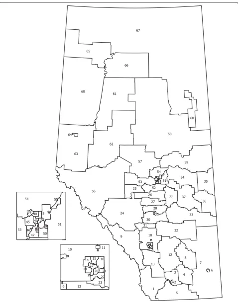
We use data from an administrative database that includes all presentations to emergency departments (EDs) in the province of Alberta, Canada. We focus on presentations to EDs for self-inflicted injuries by ado-lescents (≥ 13 and < 18 years of age) during April 1, 1998, to March 31, 1999. Individuals with at least one ED presentation during the study period are the cases and the ED presentations are the events. Data are stra-tified by sex (male, female) and age group (13-14, 15-17 years).

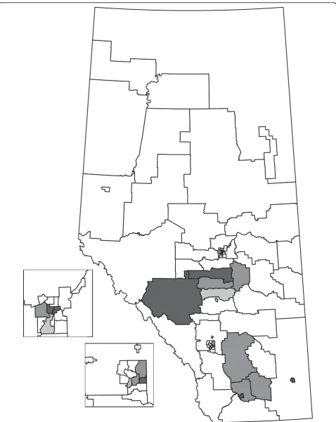
The province of Alberta (Figure 1) is divided intoI= 68 sub-Regional Health Authorities (HAs) with very diverse population sizes (median 2975, range 599 to 10298). During the study period, adolescents numbered n = 223999 in the population andc = 764 individuals presented v= 852 times to the ED with self-inflicted injuries. Although most individuals presented once, the range of presentations was one to 18. For the HAs, the median number of cases was 7.5 (range 0 to 43) and the median number of events was 8 (range 1 to 51). Alberta Health and Wellness provided the administra-tive data and the distances between population-based centroids. For each HA, Alberta Health and Wellness has determined a population-based centroid that is the latitude and longitude of the centre of the geographic area weighted by population. The distances between centroids are calculated and the ordering is provided for each cell.

Key to this illustrative example is that individuals can make multiple ED presentations during the study per-iod. If analysis is based on the cases alone and not the presentations, then a case with only one presentation and a case with 10 presentations are treated exactly the same. The information on the “extra presentations” is ignored and only areas with excess number of cases can be identified as a cluster. Areas that have excess bers of presentations, but not necessarily excess num-bers of cases, cannot be identified unless the analysis includes the presentation information. From the health services perspective, the presentations are the most appropriate unit of analysis and while identifying areas with excess cases is important, the identification of excess areas of presentations may suggest areas where disease severity may be greater or alternative health care options are not as available.

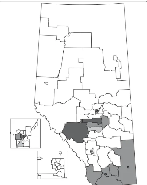
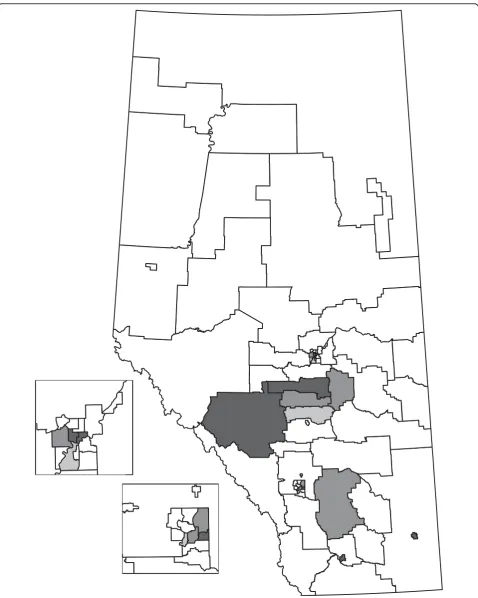
We compare the HC, CPE, and EE methods on the Alberta data set stratified by sex and age group (Table 1). The table lists the size of the cluster tested (k or k*), observed test statistic (ℓ), and the observed (O)

and expected (E) cases or events. Tests that were signifi-cant at a= 0.05 are indicated with an asterisk (*). HAs that are not significant were tested at all cluster sizes,

from w = 0 to 2, with the results for the last test

reported. For the significant HAs, the wis the same as the value of ℓ. For non-significant HAs, the number of cells (ℓ) that need to be combined to have at least the size of the cluster tested is larger thanw. The HAs are grouped according to the Regional Health Authority that provides services to the HAs (e.g., HAs 1 to 5 are part of the same Regional Health Authority). Figures 2, 3, and 4 display the HAs that are significant, either alone or in combination with other HAs. For each method, the simulation-based overall tests suggest that the results are not likely to have occurred by chance. In the 1000 simulations for the HC case analysis, 3 had at least 15 clusters observed (overallp-value = 0.003). For the event analyses, the CPE approach had 5 simulations with at least 13 clusters (overall p-value = 0.005) and the EE approach had 0 simulations with at least 15 clus-ters (overallp-value = 0.000).

The HC and EE methods both identify 15 significant HAs as part of clusters, although the significant HAs are not the same in each analysis. The CPE method identifies 13 significant HAs, all of which are identified by the EE method. Generally, the HAs that were significant with all three methods had higher numbers of cases and events than expected by chance. Similarly, the HAs that were not found to be significant by any of the methods had fewer cases and events than expected by chance. The event cluster sizes are generally very close for the EE and CPE analyses, with the EE analyses having slightly lower sizes for some HAs. One thousand Monte Carlo simula-tions were done for each method and less than six simu-lated data sets in each approach were at least as extreme as the actual number of clusters observed. Hence, not all clusters are likely to be spurious.

Table 1 Clustering results for the Alberta adolescent self-inflicted injury data from each of the three approaches

Case Analysis Event Analysis

HC CPE EE

i k ℓ O E O/E p k* ℓ O E O/E p k* ℓ O E O/E p

1 43 2 45 32.3 1.4 0.038* 51 3 51 42.6 1.2 0.154 51 3 51 42.6 1.2 0.150

2 24 0 31 16.2 1.9 0.039* 28 0 33 18.1 1.8 0.049* 28 0 33 18.1 1.8 0.048*

3 31 1 34 22.1 1.5 0.040* 44 3 50 40.9 1.2 0.332 43 2 43 30.0 1.4 0.049*

4 37 2 39 26.9 1.4 0.035* 44 3 50 40.9 1.2 0.332 43 2 43 30.0 1.4 0.049*

5 35 1 37 25.9 1.4 0.048* 50 3 50 40.9 1.2 0.134 50 3 50 40.9 1.2 0.130

6 20 0 21 12.9 1.6 0.038* 23 0 24 14.4 1.7 0.049* 23 0 24 14.4 1.7 0.048*

7 27 1 28 18.8 1.5 0.041* 41 3 41 33.3 1.2 0.143 41 3 41 33.3 1.2 0.140

8 26 5 43 42.8 1.0 0.998 31 5 48 47.7 1.0 0.989 31 5 48 47.7 1.0 0.991

9 55 5 66 82.9 0.8 1.000 65 5 77 92.4 0.8 0.996 64 5 77 92.4 0.8 0.998

10 35 4 71 77.4 0.9 1.000 41 4 80 86.3 0.9 1.000 41 4 80 86.3 0.9 1.000

11 72 3 78 76.0 1.0 0.705 85 3 91 84.8 1.1 0.479 84 3 91 84.8 1.1 0.518

12 47 3 69 70.6 1.0 0.999 36 1 42 24.0 1.8 0.046* 36 1 42 24.0 1.8 0.044*

13 90 4 97 94.9 1.0 0.722 106 4 126 105.8 1.2 0.483 105 4 126 105.8 1.2 0.519

14 69 6 111 123.6 0.9 1.000 81 6 130 137.8 0.9 1.000 81 6 130 137.8 0.9 1.000

15 84 3 92 95.1 1.0 0.901 98 3 108 106.1 1.0 0.737 97 3 108 106.1 1.0 0.780

16 73 3 78 76.8 1.0 0.695 72 1 89 54.6 1.6 0.050* 72 1 89 54.6 1.6 0.047*

17 60 4 63 83.8 0.8 0.998 71 4 73 93.4 0.8 0.981 70 4 73 93.4 0.8 0.990

18 46 3 49 61.2 0.8 0.985 55 3 59 68.2 0.9 0.921 54 3 59 68.2 0.9 0.945

19 38 3 46 54.5 0.8 0.994 46 3 52 60.8 0.9 0.957 45 3 52 60.8 0.9 0.972

20 40 3 53 56.2 0.9 0.992 48 2 49 33.6 1.5 0.044* 48 2 49 33.6 1.5 0.043*

21 73 3 91 85.5 1.1 0.935 26 0 38 16.1 2.4 0.042* 26 0 38 16.1 2.4 0.041*

22 80 3 80 76.4 1.0 0.351 94 4 125 101.3 1.2 0.720 93 4 125 101.3 1.2 0.763

23 80 3 80 76.4 1.0 0.351 94 4 125 101.3 1.2 0.720 93 4 125 101.3 1.2 0.763

24 11 0 13 5.8 2.2 0.035* 13 0 16 6.5 2.5 0.035* 13 0 16 6.5 2.5 0.034*

25 44 5 71 61.3 1.2 0.993 53 5 80 68.4 1.2 0.952 52 5 80 68.4 1.2 0.968

26 17 0 28 10.5 2.7 0.040* 20 0 31 11.8 2.6 0.043* 20 0 31 11.8 2.6 0.042*

27 32 2 36 23.2 1.5 0.046* 38 2 39 25.9 1.5 0.049* 38 2 39 25.9 1.5 0.048*

28 40 3 43 39.6 1.1 0.499 48 4 74 56.0 1.3 0.819 48 4 74 56.0 1.3 0.828

29 26 0 28 17.5 1.6 0.032* 54 5 61 55.2 1.1 0.542 54 5 61 55.2 1.1 0.545

30 41 3 42 38.7 1.1 0.378 49 5 51 65.0 0.8 0.964 49 5 51 65.0 0.8 0.969

31 38 3 43 45.6 0.9 0.896 45 4 49 58.4 0.8 0.943 45 4 49 58.4 0.8 0.949

32 37 6 38 54.7 0.7 0.996 44 7 66 80.5 0.8 1.000 44 7 66 80.5 0.8 1.000

33 27 4 29 29.7 1.0 0.722 32 5 35 41.8 0.8 0.915 32 5 35 41.8 0.8 0.921

34 27 3 29 35.6 0.8 0.946 32 4 34 44.3 0.8 0.956 32 4 34 44.3 0.8 0.961

35 25 4 34 40.3 0.8 0.997 30 4 36 44.9 0.8 0.982 30 4 36 44.9 0.8 0.984

36 26 5 26 35.5 0.7 0.962 31 6 45 58.6 0.8 1.000 30 6 45 58.6 0.8 1.000

37 27 6 54 46.0 1.2 0.999 32 6 59 51.3 1.1 0.995 32 6 59 51.3 1.1 0.996

38 25 1 32 17.5 1.8 0.049* 30 1 36 19.5 1.9 0.047* 30 1 36 19.5 1.9 0.046*

39 53 3 55 51.7 1.1 0.443 63 4 74 75.6 1.0 0.895 63 4 74 75.6 1.0 0.906

40 53 3 55 51.7 1.1 0.443 63 4 76 69.6 1.1 0.743 63 4 76 69.6 1.1 0.753

41 16 0 21 9.9 2.1 0.045* 19 0 22 11.1 2.0 0.043* 19 0 22 11.1 2.0 0.042*

42 17 0 19 10.8 1.8 0.046* 20 0 20 12.0 1.7 0.047* 20 0 20 12.0 1.7 0.046*

43 56 3 61 54.8 1.1 0.453 66 4 85 72.2 1.2 0.723 66 4 85 72.2 1.2 0.734

44 66 3 73 63.9 1.1 0.409 78 4 79 82.2 1.0 0.639 77 4 79 82.2 1.0 0.685

45 50 2 58 39.2 1.5 0.049* 60 2 62 43.7 1.4 0.045* 60 2 62 43.7 1.4 0.043*

46 51 3 54 50.4 1.1 0.484 60 3 60 56.2 1.1 0.327 60 3 60 56.2 1.1 0.324

47 45 3 54 50.4 1.1 0.803 53 3 60 56.2 1.1 0.628 53 3 60 56.2 1.1 0.634

The fact that all of the significant HAs in the CPE analysis were all identified by the EE approach is not a feature that is likely to occur in all data sets. In par-ticular, our event cluster sizes are relatively large and the relevant probabilities of the CPE and EE may be closer than in other situations. In addition, the com-pound Poisson distribution may not be an appropriate distribution for other data. Furthermore, our example had key HAs that were significant alone and when these HAs were combined with some other HAs, they too became significant. Typically, there would be some cells where the cells individually are not signifi-cant but when combined together do become significant.

In practice, a researcher would probably conduct both analyses based on cases and analyses based on events. Each analysis tests different aspects of data based on multiple disease-related events. If the median number of events is larger than one, then the analysis based on events is likely more informative. We would expect that users would prefer the EE approach over the CPE approach because it does not require distributional (parametric) assumptions, even if there is some power loss over parametric procedures. In addition, this approach can be very efficiently programmed even when there are strata variables. If there are no strata variables, then the CPE approach may be more timely.

Simulation

We examine the Type I Error of the EE and CPE approaches through simulation studies. In these studies, the Alberta cells and geographic relationship are used. The cell populations are set to be the Alberta popula-tion or the same populapopula-tion in each cell (1000, 5000, or 8000). Five settings for the probability of multiple events per case are considered (Table 2) with varying means and skewness chosen for convenience. Setting S5 is based on the self-inflicted injury data in Alberta. The event rate is set to be 2 events per 1000 population. That is, the total number of events in each simulated data set was 136, 680, and 1088 for the settings with 1000, 5000, and 8000 population per cell, respectively. When the actual Alberta population is used, the total number of events is 447. With multiple event probabil-ities and crude event rates, the simulated data sets are created by randomly assigning the c•1, c•2, ... cases to

the cells based on each cell’s proportion of the total population (as in the Monte Carlo simulations for asses-sing overall clustering). These settings allow us to demonstrate that the detection of events is different than the detection of cases. In particular, clusters of events may be identified that are not also clusters of cases.

For each simulation setting, we generated 1000 data sets and applied the CPE and EE approaches to each

Table 1: Clustering results for the Alberta adolescent self-inflicted injury data from each of the three approaches (Continued)

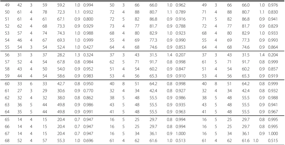
49 42 3 59 59.2 1.0 0.994 50 3 66 66.0 1.0 0.962 49 3 66 66.0 1.0 0.976

50 61 4 78 72.3 1.1 0.932 72 4 88 80.7 1.1 0.789 71 4 88 80.7 1.1 0.830

51 61 4 61 67.1 0.9 0.800 72 5 82 86.8 0.9 0.916 71 5 82 86.8 0.9 0.941

52 62 4 68 73.3 0.9 0.929 73 4 77 81.7 0.9 0.788 72 4 77 81.7 0.9 0.829

53 57 4 74 74.3 1.0 0.988 68 4 80 82.9 1.0 0.923 68 4 80 82.9 1.0 0.933

54 46 4 67 69.3 1.0 0.999 55 4 69 77.3 0.9 0.990 55 4 69 77.3 0.9 0.993

55 54 3 54 52.4 1.0 0.427 64 4 68 74.6 0.9 0.853 64 4 68 74.6 0.9 0.864

56 31 3 37 28.2 1.3 0.324 37 3 43 31.5 1.4 0.207 37 3 43 31.5 1.4 0.204

57 52 4 54 67.8 0.8 0.984 62 5 71 91.7 0.8 0.998 61 5 71 91.7 0.8 0.999

58 43 4 50 54.0 0.9 0.952 51 4 54 60.2 0.9 0.847 51 4 54 60.2 0.9 0.857

59 44 4 54 58.6 0.9 0.983 53 4 56 65.3 0.9 0.910 53 4 56 65.3 0.9 0.919

60 33 6 33 42.7 0.8 0.950 40 8 51 64.2 0.8 0.998 40 8 51 64.2 0.8 0.999

61 27 3 29 30.6 0.9 0.770 32 4 34 42.4 0.8 0.927 32 4 34 42.4 0.8 0.932

62 32 4 32 38.0 0.8 0.862 38 5 48 55.5 0.9 0.986 38 5 48 55.5 0.9 0.988

63 36 5 44 49.8 0.9 0.986 43 5 48 55.5 0.9 0.935 43 5 48 55.5 0.9 0.941

64 35 5 44 49.8 0.9 0.991 41 5 48 55.5 0.9 0.963 41 5 48 55.5 0.9 0.967

65 14 4 15 20.4 0.7 0.947 16 5 25 29.7 0.8 0.994 16 5 25 29.7 0.8 0.995

66 14 4 15 20.4 0.7 0.947 16 5 25 29.7 0.8 0.994 16 5 25 29.7 0.8 0.995

67 14 4 15 20.4 0.7 0.947 16 5 34 36.1 0.9 1.000 16 5 34 36.1 0.9 1.000

68 52 4 57 55.3 1.0 0.696 61 4 62 61.6 1.0 0.513 61 4 62 61.6 1.0 0.515

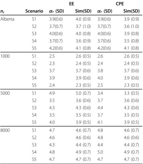
data set. To make comparisons easier, we obtained the cluster sizes {k*_i0} for each approach and tested each cell only once. The results of the simulations are shown in Table 3. With the discreteness of the distributions, the cluster size may coincide with a smaller significance level than the significance level setting of a= 0.05. We provide the effective significance level,a*, for each sce-nario based on the cluster size and provide the number of simulations that had at least one cluster detected. For the scenarios with constant cell populations thea* is the same for each simulation whereas for the data sets based on the Alberta population, the mean and standard deviation (SD) for a* are provided. As each simulated

data set has different testing results, the mean and SD for the number of significant clusters are also given.

In general, the EE and CPE approaches have similar results and the results of each approach are close to the (effective) significance level. The CPE results tend to identify slightly fewer clusters than expected. With lar-ger population sizes, the effective significance level is closer to 0.05. When the diverse population sizes of Alberta are used, the number of clusters detected is more variable. Both methods provide detection rates of false clusters that are close to what is expected by the (effective) significance level.

Conclusions

We have provided a new method for the detection of aggregations of events related to diseased individuals, called event clusters. This method builds on the approaches of Besag and Newell [3] for cases and of Rosychuk et al. [9] for events. Our approach uses the exact probability of observing events from a sample of the population. It is applicable to situations where cases may have multiple events and the number of events are of interest. The population sizes can differ from cell to cell and can be adjusted by strata. The method is easy to implement in computer code and requires a minimal amount of data from the administrative region. We used a testing algorithm similar to sequential testing to deter-mine the size of clusters specific to each cell and com-pared the new method with two other approaches using data on presentations to emergency departments for self-inflicted injuries. In some contexts, like our emer-gency department presentations, the number of events can be more relevant than the number of cases and new method provides an exact approach for determining aggregations of these events. The use of cases only does not necessarily capture the relevant type of clustering and analyses based on events can also complement ana-lyses based on cases.

Our approach is based on exact probabilities and does not require distribution assumptions as in the com-pound Poisson approach by Rosychuk et al. [9]. Those authors had to specify a probability distribution for the

Table 2 Event probabilities for the simulation scenarios

Scenario Non-zero Event ProbabilitiesQ(y)

S1 Q(1) = 0.6, Q(2) = 0.3, Q(3) = 0.1

S2 Q(1) = 0.94, Q(2) = 0.05, Q(3) = 0.01

S3 Q(1) = 0.8, Q(2) = 0.1, Q(3) = 0.05, Q(4) = 0.03, Q(5) = 0.01,

Q(6) = 0.01

S4 Q(1) = 0.8, Q(2) = 0.15, Q(3) = 0.05

S5 Q(1) = 0.929, Q(2) = 0.058, Q(3) = 0.008, Q(4) = 0.001, Q(5) = 0.001,

Q(9) = 0.001, Q(18) = 0.001

Table 3 Simulation results for each cell size and scenario

EE CPE

ni Scenario a*(SD) Sim(SD) a*(SD) Sim(SD)

Alberta S1 3.9(0.6) 4.0 (0.9) 3.9(0.6) 3.9 (0.9)

S2 3.7(0.7) 3.7 (1.0) 3.7(0.7) 3.6 (1.0)

S3 4.0(0.6) 4.0 (0.8) 4.0(0.6) 3.9 (0.8)

S4 3.7(0.7) 3.6 (0.9) 3.7(0.6) 3.5 (0.8)

S5 4.2(0.6) 4.1 (0.8) 4.2(0.6) 4.1 (0.8)

1000 S1 2.5 2.6 (0.5) 2.6 2.6 (0.5)

S2 2.3 2.4 (0.5) 2.4 2.4 (0.5)

S3 3.7 3.7 (0.6) 3.8 3.7 (0.6)

S4 3.9 3.9 (0.6) 4.0 3.9 (0.6)

S5 2.4 2.3 (0.5) 2.5 2.3 (0.5)

5000 S1 4.9 5.0 (0.7) 3.4 3.3 (0.5)

S2 3.5 3.6 (0.6) 3.7 3.6 (0.6)

S3 4.3 4.3 (0.6) 4.4 4.3 (0.6)

S4 3.5 3.5 (0.5) 3.7 3.5 (0.5)

S5 4.0 3.9 (0.5) 4.1 3.9 (0.5)

8000 S1 4.7 4.6 (0.7) 4.8 4.6 (0.7)

S2 4.6 4.6 (0.6) 4.8 4.6 (0.6)

S3 4.3 4.4 (0.7) 4.4 4.4 (0.7)

S4 4.8 4.9 (0.7) 5.0 4.9 (0.7)

S5 4.7 4.7 (0.7) 4.7 4.7 (0.7)

situation when a case has exactly yevents and use esti-mates in their application. The distribution could be misspecified, estimates may not be very precise, and the p-value does not capture the additional uncertainty of these estimates. Our method uses the multiple hyper-geometric distribution that does require a distribution, or estimates, for the event probabilities. Our new approach is particularly appealing when analyses are conducted by strata variables. With more strata vari-ables, there are fewer possible combinations to calculate and the use of convolutions makes the computational time less than that required by the compound Poisson approach.

One drawback of the testing algorithm is that the user must choose the number of cluster sizes to be tested. This choice is perhaps easier than choosing a particular cluster size to test, especially if areas have diverse popu-lation sizes. Furthermore, the structure of the algorithm dictates that statistically significant cells will have the unappealing feature that p-values will be close to the significance level. Additionally, overall clustering can be assessed through Monte Carlo simulations and the same approach could be used to examine individual cell tests (i.e., calculate the proportion of simulations for which a particular cell was statistically significant as described in Rosychuk et al. [9]).

Both our new method and the compound Poisson method require that the number of events per cases is known. We also introduced an approach for the situa-tion when the number of cases and events are known, but not the number of events for each case. Administra-tive data sources may not record the number of events per case and we provided an analysis approach for this context. This approach considers events to be indistin-guishable and does not specifically use the number of cases. While not preferable to the analysis with informa-tion on the events per case, this approach is applicable for less detailed administrative data.

Further work is necessary to compare the power of the different approaches to detect different sized clusters and to consider different data generating mechanisms. Most cases in our data example only had one event. Our event results were different than the case analysis but further examination should include larger numbers of events per case. Such investigations will give users a greater ability to decide which method is most appropri-ate for the surveillance of disease-relappropri-ated events in their jurisdiction.

Acknowledgements

This work was supported by a research grant from the Canadian Institutes of Health Research (R.J.R.) and salary support from the Alberta Heritage Foundation for Medical Research (AHFMR; Edmonton, AB; R.J.R.). The funding bodies did not have any role in the study design; in the collection analysis,

and interpretation of the data; in the writing of the manuscript; and in the decision to submit the manuscript for publication. The authors thank Alberta Health and Wellness for providing the data.

Author details

1_{Department of Pediatrics, 11402 University Avenue NW, Edmonton, Alberta,}

Canada.2Women and Children’s Health Research Institute, Edmonton, Alberta, Canada.3_{Department of Chemistry, 200 University Avenue West,}

Waterloo, Ontario, Canada.

Authors_’contributions

RJR developed created the methodology, performed the analysis, and wrote the initial draft of the manuscript. JLS developed and coded the efficient algorithm for all computations and revised the manuscript. All authors read and approved the final manuscript.

Competing interests

The authors declare that they have no competing interests.

Received: 27 December 2009 Accepted: 7 June 2010 Published: 7 June 2010

References

1. Lawson A, Biggeri A, Böhning D, Lesaffre E, Viel JF, Bertollini R:Disease Mapping and Risk Assessment for Public Health West SussexUK: John Wiley & Sons Ltd 1999.

2. Waller LA, Gotway CA:Applied Spatial Statistics for Public Health Data HobokenNJ: John Wiley & Sons Ltd 2004.

3. Besag J, Newell J:The detection of clusters in rare diseases.Journal of the Royal Statistical Society, Series A1991,154:143-155.

4. Openshaw S, Charlton M, Craft AW, Birch JM:Investigation of leukaemia clusters by use of a geographical analysis machine.Lancet1988,

331:272-273.

5. Turnbull BW, Iwano EJ, Burnett WS, Howe HL, Clark LC:Monitoring for clusters of disease: Applications to leukemia incidence in Upstate New York.American Journal of Epidemiology1990,132:S136-S143.

6. Kulldorff M, Nagarwalla N:Spatial disease clusters: detection and inference.Statistics in Medicine1995,14:799-810.

7. Duczmal L, Assunção R:A simulated annealing strategy for the detection of arbitrarily shaped spatial clusters.Computational Statistics and Data Analysis2004,45:269-286.

8. Tango T:A class of test for detecting‘general’and‘focused’clustering of rare diseases.Statistics in Medicine1995,14:2323-2334.

9. Rosychuk RJ, Huston C, Prasad NGN:Spatial Event Cluster Detection Using a Compound Poisson Distribution.Biometrics2006,62:465-470.

10. Rosychuk RJ, Colman I, Rowe BH:Comparison of cluster detection using patients and events of medically treated self-inflicted injuries in Alberta, Canada.Heath Services and Outcomes Research Methodology2009,

9:100-116.

11. Feller W:An Introduction to Probability Theory and Its ApplicationsNew York, NY: John Wiley & Sons, Inc, 3 1968,1.

12. Le ND, Petkau AJ, Rosychuk RJ:Surveillance of Clustering Near Point Sources.Statistics in Medicine1996,15:727-740.

doi:10.1186/1476-072X-9-28