A. Heibig, F. Filbet, L. I. Palade, Editors
MATHEMATICAL FRAMEWORK FOR TRACTION FORCE MICROSCOPY
R. Michel
1, V. Peschetola
1,2, G. Vitale
3, J. ´
Etienne
1, A. Duperray
4,5,
D. Ambrosi
6, L. Preziosi
2et C. Verdier
1R´esum´e. Cet article est consacr´e au probl`eme de la Microscopie `a Force de Traction (TFM). Ce probl`eme consiste `a d´eterminer les contraintes exerc´ees par une cellule lors de sa migration sur un substrat ´elastique `a partir d’une mesure exp´erimentale des d´eplacements induits dans ce substrat. Math´ematiquement, il s’agit de r´esoudre un probl`eme inverse pour lequel nous proposons une formu-lation abstraite de type optimisation sous contraintes. Les contraintes math´ematiques expriment les constraintes biom´ecaniques que doit satisfaire le champ de contraintes exerc´e par la cellule. Ce cadre abstrait permet de retrouver deux des m´ethodes de r´esolution utilis´ees en pratique, `a savoir la m´ethode adjointe (AM) et la m´ethode de Cytom´etrie de Traction par Transform´ee de Fourier (FTTC). Il per-met aussi d’ameliorer la m´ethode FTTC. Les r´esultats num´eriques obtenus sont ensuite compar´es et d´emontrent l’avantage de la m´ethode adjointe, en particulier par sa capacit´e `a capturer des d´etails avec une meilleure pr´ecision.
Abstract. This paper deals with the Traction Force Microscopy (TFM) problem. It consists in obtaining stresses by solving an inverse problem in an elastic medium, from known experimentally measured displacements. In this article, the application is the determination of the stresses exerted by a living cell at the surface of an elastic gel. We propose an abstract framework which formulates this inverse problem as a constrained minimization one. The mathematical constraints express the biomechanical conditions that the stress field must satisfy. From this framework, two methods currently used can be derived, the adjoint method (AM) and the Fourier Transform Traction Cytometry (FTTC) method. An improvement of the FTTC method is also derived using this framework. The numerical results are compared and show the advantage of the AM, in particular its ability to capture details more accurately.
Key words. Cell motility, Inverse problems, Tikhonov regularization, Adjoint Method (AM), Fourier Transform Traction Cytometry (FTTC),L–curve.
1
CNRS / Univ. Grenoble 1, Laboratoire Interdisciplinaire de Physique, UMR 5588, Grenoble, F-38041, France.
2
Dipartimento di Matematica, Politecnico di Torino, 10129 Torino, Italy.
3
Laboratoire de M´ecanique des Solides, CNRS UMR 7649, ´Ecole Polytechnique, 91128 Palaiseau Cedex, France.
4
INSERM U823, Grenoble, France.
5
Univ. Grenoble 1, Institut Albert Bonniot et Institut Fran¸cais du sang, UMR-S823, Grenoble, France.
6
MOX - Dipartimento di Matematica, Politecnico di Milano, Milano, Italy.
©EDP Sciences, SMAI 2013
1.
Introduction
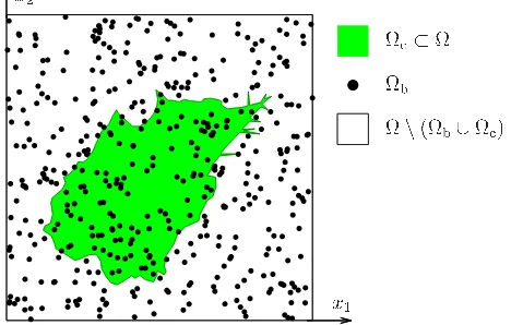
Living cells have the ability to migrate on different 2D–susbstrates which are considered to be in vitro model for understanding cell motility. Indeed, cells pull on the substrate and can deform it by developing forces, which are called traction forces. It is essential to determine such forces, because one can then understand how cells regulate their adhesion and modify their cytoskeleton [4] in order to produce such a complex process, i.e. migration. To determine traction forces or more precisely traction stresses, assuming that cells do not penetrate into the substrate, biophysicists have proposed to use beads embedded in the substrate [11]. By following the positions of beads, as compared to their initial state, one obtains displacements in the migration plane. These displacements are denoted byuband are defined on a part Ωb of the whole computational domain (see Fig. 1 below). They are related to the stresses applied by cells by the elasticity problem. So, the determination of the traction stress field from the (partial) knowledgeubof the induced displacements needs to solve aninverse elasticity problem. This method has been called Traction Force Microscopy (TFM) and has been considered using different formulations, the BEM (Boundary Element Method (BEM) [11], the Fourier Transform Traction Cytometry (FTTC) method [8], the Traction Recovery from Point Force (TRPF) [22], and finally the more recent Adjoint Method (AM) [2, 3, 25].
An important point, sometimes neglected in the literature, is the fact that the traction stress field must satisfy a set ofbiomechanical constraints. First, the cell is not in contact with the substrate on the whole computational domain, but only over a subdomain denoted by Ωc and called the cell domain (see Fig. 1 below). Therefore
Figure 1. Schematic representation of the computational domain. Ω: 2D computational domain corresponding to the cell migration plane; Ωc: cell domain, the part of Ω “below” the cell; Ωb: beads domain. See also Fig. 2 page 70.
stresses are zero outside this cell domain. Next, if the cell moves slowly (as is the case) or in a quasistatic way, it is in equilibrium and the sum of forces and moments vanish. This can be written in mathematical terms as:
supp (T)⊂Ωc, Z
Ωc
Tdx= 0 and Z
Ωc
x∧Tdx= 0 (1)
After the seminal paper of Demboet al.[11] the FTTC method [8] has been proposed as a simpler framework and more efficient in terms of computational time. Nevertheless, the FTTC method does not allow to impose the zero moment constraint and needs to be modified to account for one of the biomechanical conditions, the localization constraint which imposes no stresses outside the cell domain. A way to impose this localization constraint, called constrained–FTTC, has been proposed [8], but, to the best of our knowledge, it seems that this variant has never been used. In this work, we focus on the localization condition and we propose an improvement of the classical FTTC method to satisfy this constraint.
By contrast, the adjoint method does not have any difficulty to impose the biomechanical constraints (1). The localization constraint was imposed in [2], then the zero force constraint was taken into account [20]. More recently [25], the zero moment constraint was also imposed. This method could be thought of as a tool to differentiate different cells, in particular cancer cells with different invasiveness [2, 3, 19].
The outline of this paper is as follows. In the next section, we present an abstract variational framework which allows to formulate the TFM problem as a constrained minimization problem. In order to insure uniqueness and regularity of the solution, a regularization term is added to the objective function. This framework is used in section 3 to derive the adjoint method and in section 4 to improve the FTTC method in order to meet the localization constraint. In section 5, the issue of the choice of the regularization parameter is discussed and the traction stresses fields obtained by using adjoint method and improved FTTC method are compared in a real case.
2.
Abstract variational framework for the TFM problem
In this section we define an abstract variational framework to formulate and solve the TFM problem. The functional framework is described in section 2.1 in terms of spaces and operators. Then, in section 2.2, we define the unknown traction stress field as the solution of a constrained minimization problem. Next, in section 2.3 we reformulate the optimal conditions as a set of unconstrained variational equations involving the adjoint state and the displacement field as unknowns. The traction stress field is then obtained by using a projection operator. Finally, in section 2.4 we summarize some classical results concerning the convergence of the regularization process.
2.1.
Functional framework
Spaces. LetH be a real Hilbert space. We denote by (·,·)H its scalar product and by ||·||H =
p
(·,·)H the corresponding norm. LetV ⊂H be a linear subspace of H. We assume thatV is dense inH for the topology induced by the norm||·||H(V
H
=H), and that, equipped with its own norm||·||V,V is a reflexive Banach space such that the injection from V intoH is continuous (V H). Under these conditions, the canonical injection from the spaceH into its dualH′ defines a linear continuous injective operator whose range is dense inH′ [7].
If, by using the Riesz theorem, we identify H with its dual H′ (H ≡H′, that isH is chosen aspivot space for
the duality pairing), then the spacesV,H andV′ form aGelfand triple:
V H ≡H′ V′ with VH=H and H′V′=V′ (2)
Furthermore, the duality pairing satisfies the following relations
hT,SiH′,H = (T,S)H ∀(T,S)∈H×H and hT,viV′,V = (T,v)H ∀ (T,v)∈H×V (3)
spaces. The first one isHc a closed non empty subspace ofH related to biomechanical constraints, (or at least some of these constraints), and the second one is Xb, another real Hilbert space related to the experimentally measured displacementsub. Depending on the used formulation and on the nature ofub, Xb is either a finite dimensional space (see the section 4.4, or the formulation used in [25]), either a closed non empty subspace ofH (whenubis a function and Ωb an open set). In both cases, we denote by (·,·)Xb and||·||Xb the scalar product
and its associated norm in Xb. Note that under these conditions, the spaceXbcan be identified with its dual space without contravening with the choice of the space H as pivot space.
Elasticity operator. The relationship between the stress field T imposed by the cell during its migration and the displacement u induced in the gel (on the gel surface) is represented by a continuous linear operator A∈L(V, V′) fromV into its dual V′. We assume theAisV-elliptic in the sense that:
∃α >0 such that hAv,viV′,V ≥α||v||
2
V ∀v∈V (4)
Under these conditions,A is bijective. Furthermore, sinceV andV′ are two Banach spaces, thanks to Banach
theorem, the inverse A−1 is a linear continuous operator from V′ into V. Thus, A∈Isom(V, V′) and A−1 ∈ Isom(V′, V). Hence, all stress fields T imposed by the cell and the induced displacements u in the gel are
related by:
Au=T in V′ ⇐⇒ u=A−1T inV (5)
In addition, the adjoint operator AT is also an isomorphism and, thanks to reflexivity of V, we have AT ∈ Isom(V, V′) andA−T∈Isom(V, V′) whereA−Tdenotes the inverse of AT.
Observation operator and data. To compare the theoretical displacementsu=A−1T ∈V to the experi-mental beads displacements ub∈Xbwe use a continuous linear operator B ∈L (V, Xb) which can be viewed as theobservation operator. This comparison involves theresidual vector BA−1T−u
b∈Xb. As Xb can be identified with its dual, we haveBT∈L(Xb, V′).
2.2.
The TFM problem as a constrained minimization problem
Tikhonov functional. Given a positive real-valued parameter ε > 0, we define the so–called Tikhonov functional Jε:T ∈H 7−→Jε(T)∈R+ by
Jε(T) = 1 2
BA−1T−ub 2
Xb+
ε 2||T||
2
H (6)
The following two propositions establish the differentiability and convexity properties that are needed.
Proposition 2.1(Differentiability).The Tikhonov functionalJε(·)defined by(6)is twice Frechet–differentiable everywhere in H and, for all T ∈H, its first and second derivativesJ′
ε(T)∈ H′ and Jε′′(T)∈L(H×H,R) read
hJ′
ε(T),δTiH′,H = BA
−1T−u
b, BA−1δTXb + ε(T,δT)H (7) hJε′′(T),(δT,δS)iH′,H = BA
−1δT, BA−1δS
Xb + ε(δT,δS)H (8)
for all(δT,δS)∈H×H.
Proof. Direct computation and application of the Frechet derivative definition.
Proof. From equation (8), we have hJ′′
ε(T),(δT,δT)iH′,H =
BA−1δT2
Xb + ε||δT||
2
H ≥ ε||δT||
2
H for allδT ∈H. So, sinceε >0,J′′
ε(T) is H–elliptic for allT ∈ H. Then, the Tikhonov functional Jε is strictly
convex everywhere overH [10].
Now, we can define rigorously the required stress fieldTεas the solution of the following constrained minimiza-tion problem.
Probl`eme 2.3. (Constrained minimization problem) Givenub∈Xb, andε >0, findTε such that Tε∈Hc and Jε(Tε) = min
T∈Hc
Jε(T) (9)
This problem is well-posed in the sense that the following theorem holds.
Th´eor`eme 2.4. The constrained minimization problem 2.3 has one and only one solution Tε which satisfies the following variational equation
Tε∈Hc and BA−1Tε−ub, BA−1TXb + ε(Tε,T)H = 0 ∀T ∈Hc (10)
Proof. The Tikhonov functionalJεis strictly convex everywhere inH(cf. prop. 2.2), andHcis a closed subspace of the Hilbert space H, so [7, 10], the minimization problem 2.3 has one and only one solution Tε ∈ Hc. Moreover [7, 10], this solution satisfies the Euler equation hJ′
ε(Tε),TiH′,H = 0 ∀T ∈ Hc which, by using definition (7) ofJ′
ε(Tε), is rewritten as (10).
The definition (6) of the Tikhonov functional Jε(·) involves two terms. The first one, the residual norm
BA−1T −u b
2
Xb, measures the goodness of the optimal solution Tε, i.e. its ability to predict the
experi-mental displacementsub. Qualitatively, if this term is too large,Tεcannot be considered as a suitable solution. But a small value is not necessarily a satisfying condition to meet. Indeed, when a small value of the residual norm occurs, then uncertainties in the data ub take too much weight. As a result, the solution Tε is domi-nated by high–frequency components with large amplitudes and becomes so irregular that it looses its physical meaning. It is the well known instability of the inverse problem solution [14, 16]. So, the second term in the definition of Jε(·), the stress norm||T||2H, measures the regularity of the optimal solution Tε. Its role is to restore and enforce the stability ofTεby penalizing its norm. The Tikhonov functional can be understood as a balance between two contradictory requirements: obtaining small residuals with a sufficiently smooth solution. Theregularization parameter εcan be viewed as a tuning parameter for this balance. Large values of εlead to very smooth stress fields with poor residuals. Conversely, smaller values ofεgive good residuals with unrealistic stresses. In section 5, we deal with the manner to choose this regularization parameter.
Another way to regularize the TFM problem is to apply a low-pass filtering in order to avoid the high-frequency components in the experimental beads displacements [24].
2.3.
Solving the TFM problem
Adjoint state. By using the definition of the adjoint operator and the property (3) of the duality pairing, we can reformulate theXb–scalar product involved in the variational equation (10) as follows
BA−1T
ε−ub, BA−1TXb = BT BA−1Tε−ub, A−1TV′,V = A−TBT BA−1T
ε−ub,TV,V′
= A−TBT BA−1T
ε−ub,TH Note that this derivation uses explicitely the identification of the space Xbwith its dualXb′.
By substituting this last identity in the variational equation (10), we obtain another equivalent characterization of the optimal stress fieldTε
Tε∈Hc and A−TBT BA−1Tε−ub,TH + ε(Tε,T)H = 0 ∀T ∈Hc (11) SinceBT∈L(Xb, V′),BT BA−1T
ε−ubbelongs toV′, andAT∈L(V, V′) is an isomorphism fromV into its dualV′, there exists one and only one element p
εsuch that
pε∈V and ATp
ε=BT BA−1Tε−ub in V′ (12)
This fieldpε∈V is the classical adjoint state [18] applied to the TFM problem.
Interpretation of the optimal condition and projection operator. The adjoint state pεcan be viewed as a simple auxiliary unknown which allows us to rephrase the characterization equation (11) ofTε. Indeed, by substituting the adjoint equation (12) into (11) we obtain
Tε∈Hc, pε∈V and (pε+εTε,T)H = 0 ∀T ∈Hc (13)
This new variational equation is nothing but the characterization of−εTε∈Hc as theprojection of the adjoint statepε∈V (as an element of H) onto the biomechanical constraints spaceHc [7, 10], that is:
Tε = − 1
εPcpε inH (14)
where Pc is the projection operator from H onto Hc with respect to the scalar product (·,·)H. Since Hc is a linear subspace ofH, Pc is a linear continuous operator from H into H (Pc ∈ L(H, H)), furthermore, Pc is self–adjoint (PT
c =Pc) and idempotent (PcPc=Pc).
Three fields problem. As Tε ∈H, by using the injection H V′ involved by the Gelfand triple (2), Tε also belongs toV′. So we can define the displacement field u
εrelated to the stress field Tεand defined as the solution of
uε∈V and Auε=Tε in V′ (15)
Obviously, existence and uniqueness follow from A∈ Isom(V, V′). Next, by substituting Tε forAuε we can rewrite the adjoint equation (12) as
pε∈V and ATpε=BT(Buε−ub) in V′
On the other hand, by taking into acount (14) we reformulate (15) as a relationship betweenuε andpε
uε∈V and Auε=−1εPcpε inV
′ (16)
Probl`eme 2.5. (Three fields problem) Givenub∈Xbandε >0, find (pε,uε,Tε)∈V ×V ×Hc such that 1. (pε,uε)∈V ×V is the solution of
1
εPcpε + Auε = 0 in V
′ (17a)
ATpε − BTBuε = −BTub in V′ (17b) 2. then, deduceTε∈Hc by
Tε=− 1
εPcpε inH (17c)
This problem is well–posed and allows to solve the constrained minimization problem 2.3 as proved by the following theorem.
Th´eor`eme 2.6. The three fields problem 2.5 has one and only one solution. Furthermore, the component Tε of this solution is also the solution of the constrained minimization problem 2.3.
Proof. Existence. The theorem 2.4 establishes the existence ofTε∈Hc which solves the constrained minimiza-tion problem 2.3. So, starting from this existence result forTε, we can reproduce integrally the above discussion to establish the existence of a solution (pε,uε,Tε)∈V ×V ×Hc of the problem 2.5 such that its component
Tεsolves the problem 2.3.
Uniqueness. Since the equations (17) are linear, to show uniqueness of their solution it is sufficient to show that the only solution of (17) corresponding toub= 0 is (pε,uε,Tε) = (0,0,0). So, let (pε,uε,Tε)∈V ×V ×Hc be a solution of equations (17) corresponding to ub= 0. If ub = 0, since AT∈ Isom(V, V′), equation (17b) yieldspε=A−TBTBuε. Thus, equation (17c) can be rewritten as
PcA−TBTBuε + ε Auε = 0
By definition of the projection operator Pc (fromH ontoHc in the sense of (·,·)H) and becauseHc is a linear space, we deduce that
A−TBTBu
ε + ε Auε,T
H= 0 ∀T ∈Hc and Auε∈Hc
Thus, we can chooseT =Auεin the previous variational equation and obtain
A−TBTBu
ε + ε Auε, Auε
H = 0
By applying the definition of the adjoint operatorsATandBT, this last equation leads to
||Buε||2Xb+ε||Auε||
2
H = 0
Since ε > 0, it then follows that Auε = 0 in H. So (Auε,T)H = 0 for all T ∈ H, and since V H, in particular holds forT =uε. According to (3) we have (Auε,uε)H=hAuε,uεiV′,V and theV–ellipticity (4) of
Remarque 2.7. When the projection operatorPc is explicitely known, equations (17) can be directly used to define a numerical method to approximate the optimal solutionTε. Indeed, under these conditions equations (17a) and (17b) a explicitely define an unconstrained problem and then the pε–component of its solution can be explicitely calculated by using the projection step (17c). This situation occurs when only the localization constraint and the zero force constraint are imposed in the constrained space [20] (see (24) and (25) in the next section). This is precisely the situation in which the adjoint and FTTC methods can be compared.
When the zero moment constraint is also taken into acount, the projection operator Pc exists but not in an explicit form. So, the problem 2.5 remains only a theoretical one. To obtain a theoretical formulation which can produce a numerical method, it is better to impose the zero moment constraint by duality [25] using a Lagrange multiplier.
2.4.
Convergence propertries
In this section, we consider the behavior of the family (Tε)ε>0 of Tikhonov solutions when the regularization parameterεvaries. This section is a concise account of classical results [12,16]. More recent and specific results can be found for instance in [6].
In practice, experimental bead displacementsub∈Xbare never known exactly. They are only an approximation of the exact bead displacementsub,exact∈Xband there exists anoise level δ >0 such that
||ub−ub,exact||H≤δ (18)
For instance, the uncertainly on the experimental data used in section 5 allows us to estimate the noise level around 0.03µm for displacements of a few micrometers. This noise levelδplays a crucial role in the convergence
of the familly (Tε)ε>0as ε−→0.
A first consequence of the presence of noise in the experimental data is that, in general, we cannot assume that the bead displacements ub are in the rangeR BA−1of the operatorBA−1. Moreover, the observation operator B is not injective. Hence, in order to analyse the convergence properties of the familly (Tε)ε>0, it is convenient to introduce the Moore–Penrose generalized inverse BA−1+ of BA−1 [12] and to define the so-calledbest-approximate solution T+ as the field
T+ = BA−1+u
b,exact=AB+ub,exact
whereB+ denotes the Moore–Penrose generalized inverse of the observation operatorB. Let us define the regularized solutionTε,exactrelated to the exact bead displacements as
Tε,exact∈Hc and Jε,exact(Tε,exact) = min T∈Hc
Jε,exact(T)
where the functionalJε,exact(·) is defined in the same manner than the Tikhonov functional (6) withub,exactin place ofub.
Then, the convergence of the familly (Tε)ε>0 toT + asε
−→0 can be expressed by the following estimate
Tε−T+
H ≤
Tε,exact−T+
H+||Tε−Tε,exact||H
Tε,exact−T+H=O(εµ) with a constantµ∈]0,1] depending on the particular form of the operatorA. Thus, we have the following convergence estimate
Tε−T+H ≤ C εµ + √δ
ε with µ∈]0,1] and C >0 (19)
In the ideal but highly unlikely case when the bead displacements are known exactly, the estimation (19) establishes the convergence of theTεto the best-approximate solutionT+. In the more realistic case when the bead displacements are known only up to an error ofδ >0 in the sense of (18), the estimate (19) shows that:
(i) the fieldTε calculated using the Tikhonov method explodes asε−→0; (ii) Tε−T+
H cannot converge to zero;
(iii) the miminal value of the error normTε−T+
H is achievable only if the regularization parameterε is chosen as a function of the noise levelδin order to minimize the right hand side of the estimate (19); (iv) under this last optimal choice ε(δ), Tε(δ) converges to the best-approximate solution T+ as the noise
levelδtends to zero.
The statement (i) is illustrated by the curves shown in Fig. 5. We have chosen the value of the regularization parameter defined in the statement (iii) using an exploration of theL–curve as described in section 5.
3.
Adjoint method
Basically, applying the adjoint method to the TFM problem consists in solving a specific form of the equations (17) involved in the problem 2.5. A specific form is achieved by choosing a particular operator Ainvolved in the direct problem (5). This operator expresses the weak form of a boundary value problem describing the interactions between a cell and the gel during cell migration. In this section, we start to reduce the direct problem to a 2D boundary value problem defined on the gel surface Ω. Next, we apply the theory described in section 2 in order to recover the original adjoint method applied to the TFM problem [2] and its variant obtained by taking into account the biomechanical constraints of zero resultant force [20].
In order to compare numerically the adjoint method with the FTTC method, we restrict the biomechanical constraints taken into account to the localization constraint (supp (T) ⊂ Ωc) and the zero resultant force (RΩcTdx= 0). Indeed, to the best of our knowledge, the FTTC method does not allow to impose the zero moment constraint (RΩcx∧Tdx= 0).
3.1.
Reduction to a 2D problem
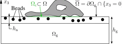
Geometry and active layer. The gel domain is modeled by the parallelepiped Ωg = Ω×]−hg,0[ in the Euclidian spaceR3with cartesian coordinates (x1, x2, x3) = (x, x3). Ω⊂R2 is the gel surface, that is the part of the boundary∂Ωg on which the cell migrates, andhgis the gel thickness in thex3direction. The horizontal extension of Ωg is about 2 mm while its vertical one is about 70µm. So, from a mechanical point of view, Ωg
can be considered as a thin plate. In addition, we assume that (i) the body (gravity) and inertial forces are negligible in the whole Ωg in comparison with the forces exerted by the cell, (ii) the vertical displacementd3 is negligible in comparison with the horizontal onesd1 andd2 and (iii) the cell exerts only tangential stresses on the gel surface Ω. Under these assumptions and using dimensional analysis, Ambrosi shows [2], first that there exists an active layer beyond which the horizontal displacements d1 and d2 vanish, and, second, that in the whole Ωgtheσ33component of the stress tensor can be neglected in comparison with the shear stresses exerted by the cell on the surface Ω. In mathematical terms, we have
whereha denotes the thickness of this active layer. All these geometrical concepts are sketched in figure 2.
cell Beads
hg x3
ha
Ωg
Ωc⊂Ω Ω =∂Ωg∩ {x3= 0}
Figure 2. Schematic representation of a cell on the elastic substrate. Ωg: 3D elastic subtrate; Ω: 2D calculation domain corresponding to the cell migration plane (Ω is the interior of∂Ωg∩ {x3= 0}); Ωc: cell domain, the part of Ω “below” the cell. See also the Fig. 1 page 62.
As a consequence, the first hypothesis leads to vanishing of the componentsσ13 andσ23below the active layer, that is
σα3 ≈ 0 in Ω×]−hg,−ha[ forα= 1,2 and the second one allows us to use the plane stress approximation.
From these observations, it is possible to reduce the TFM problem to a 2D problem by using a vertical average of fields and equations across the active layer.
Depth-averaged model. The depth–averaged operator is (formally) defined as the map which associates to the function ϕ : (x, x3) ∈ Ωg 7−→ ϕ(x, x3) ∈ R the function ϕ : x ∈ Ω 7−→ ϕ(x) ∈ R such that ϕ(x) = 1
ha
R0
−haϕ(x, x3)dx3. By applying this operator to the 3D stress equilibrium equations related to
directionsx1 andx2, and by combining with the plane stress approximation of the 3D Hooke’s law for isotropic and homogeneous material, we can express the relationship between the depth–averaged displacementsuα=dα and the cell traction stressT as
divσ(u) + T = 0 in Ω (20a)
σ(u) = 2µ2dε(u) + λ2ddivu I in Ω (20b)
ε(u) = 1
2 ∇u + ∇u
T in Ω (20c)
u = 0 on ∂Ω (20d)
whereλ2dandµ2d are the 2D Lam´e’s coefficients defined by µ2d=ha
E
2(1 +ν) and λ2d=ha ν E 1−ν2
withE andν denote respectively the Young modulus and Poisson ratio of the substrate.
3.2.
Direct problem
Functional spaces. The spaces H for traction stresses and V for gel displacements are chosen in order to define the solution of the boundary value problem (20) in the weak sense. Thus we use usual Lebesgue and Sobolev spaces
H =L2(Ω) =L2(Ω) ×L2(Ω) and V =H10(Ω) =H01(Ω) × H01(Ω) equipped with their usual scalar products [1, 7], that is (u,v)H = (u,v)L2
(Ω) = R
Ωu·vdx and (u,v)V = (u,v)H1
0(Ω) =
R
Ω∇u: ∇vdx where ∇u: ∇v = Σi,j∂jui∂jvi. Therefore, we have V
′ = H−1(Ω) = H−1(Ω) × H−1(Ω) and the Gelfand triple property (2) holds [1, 7].
Direct problem. The elasticity operatorA results from the weak form of the boundary value problem (20). Therefore, if we define the bilineara(·,·) onH10(Ω)×H10(Ω) by
a(u,v) = 2µ2d Z
Ω
ε(u) :ε(v) dx + λ2d Z
Ω
divudivvdx ∀u,v∈H10(Ω) (21a)
we choose the operator Aas the element ofL H1
0(Ω),H−1(Ω)
defined by
hAu,viV′,V = a(u,v) ∀u,v∈H
1
0(Ω) (21b)
The direct problem related to this operator is well-posed as it is showed in the following proposition.
Proposition 3.1. The elasticity operator defined by (21) satisfies the H10(Ω)–ellipticity condition (4) and defines a self-adjoint isomorphism from H10(Ω) toH−1(Ω): A∈Isom H10(Ω),H−1(Ω)
andAT=A.
Proof. TheH10(Ω)–ellipticity results from the classical Korn inequality [9] and then the isomorphism property results from the Lax-Milgram lemma [7]. The self-adjonction of A is a direct consequence of the definition
(21).
3.3.
Observation operator
Data space and observation operator. We assume that the data is continuous in the sense that experimental beads displacementsubare known in a subset Ωb(Ω which has a non zero Lebesgue measure (|Ωb|>0). The case of pointwise data is considered in [25]. So the data ub must be at least a function defined on Ωb. But, as indicated in section 2, the spaceXb must be a Hilbert space which can be identified with its dual without contravening to the identificationL2(Ω)′≡L2(Ω). To meet these requirements, we define the Hilbert spaceXb as the following closed subspace ofL2(Ω)
Xb = v∈L2(Ω) ; supp (v)⊂Ωb (22) and the value taken by the observation operatorB when evaluated at v∈H10(Ω) as
Bv : x∈Ω7−→(Bv) (x) =χb(x)v(x)∈R2 (23) where χb(·) stands for the characteristic function of the subset Ωb (χb(x) = 1 if x ∈ Ωb and χb(x) = 0 if
x∈Ω\Ωb). Thanks to the Poincar´e inequality [1, 7], it is clear that B ∈L H10(Ω), Xb. But, there exists another way to interpret the operator B, a way that will allow to simplify the application of equations (17).
(1) B is the restriction toH10(Ω) of Pb, that is B=Pb|H1 0(Ω);
(2) B is self–adjoint (BT=B) and idempotent (BB=B).
Proof. AsXbis a closed subspace ofL2(Ω), the value of Pb evaluated atv ∈L2(Ω) is characterized by [7, 10] Pbv∈Xband (v−Pbv,ϕ)L2
(Ω)= 0∀ϕ∈Xb. Hence, it is easy to verify thatPbv is defined as the function Pbv : x∈Ω7−→(Pbv) (x) =χb(x)v(x)∈R2. By comparison with definition (23) the first point holds. The second point is a property of the projection onto a closed subspace.
3.4.
Constrained space and projection operator
Constrained space and projection operator. As indicated in the introduction of this section, we restrict the set of biomechanical constraints to the ones that the FTTC method can handle. Thus, we choose the constrained spaceHc as
Hc =
T ∈L2(Ω) ; supp (T)⊂Ωc and Z
Ωc
Tdx= 0
(24)
It is clear thatHc is a closed subspace ofL2(Ω).
To use the abstract equations (17), it remains to identify the projection operatorPc.
Proposition 3.3(Structure of the projection operator). The projection operatorPc belongs to the space L L2(Ω),L2(Ω)and for allT ∈L2(Ω), the elementPcT is characterized by
PcT : x∈Ω7−→(PcT) (x) =χc(x) (T(x)−TΩc) ∈ R
2 (25a)
whereTΩc andχc(·) denote respectively the average value ofT overΩc and the characteristic function ofΩc
TΩc=
1 |Ωc|
Z
Ωc
Tdx and χc(x) =
1 if x∈Ωc
0 if x∈Ω\Ωc (25b) Proof. The proof is very similar to proof of proposition 3.2. First, the function PcT defined by (25a) belongs to the space Hc defined in (24). Next, for all ϕ ∈ L2(Ω) we have (T−PcT,ϕ)L2
(Ω) = (TΩc,ϕ)L2(Ωc) =
|Ωc|TΩcϕΩc. So, if we chooseϕin the space Hc, we can write that (T−PcT,ϕ)L2(Ω) = 0 ∀ϕ∈Hc. Hence,
the functionPcT defined by (25a) is theL2(Ω)–orthogonal projection ofT ∈L2(Ω) onto the constrained space
Hc.
3.5.
Solving the TFM problem by using adjoint method
By combining the results of the current section with the theory developed in section 2, we can develop the direct formulation of the TFM problem 2.5 with the constrained spaceHc and the data spaceXbrespectively defined by (24) and (22).
Probl`eme 3.4. (Direct formulation of the TFM) Givenub∈Xbandε >0, find (pε,uε)∈H10(Ω)×H10(Ω) solution of the following variational equations
a(pε,q) − Z
Ω
χbuε·qdx = − Z
Ω
χbub·qdx ∀q∈H10(Ω) (26a) 1
ε
Z
Ω
χcpε·vdx − 1 ε
1 |Ωc|
Z
Ωc
pεdx
Z
Ω
where the bilinear forma(·,·) is defined in (21). Then, deduceTε∈Hc by
Tε=− 1 ε
χcpε − 1 |Ωc|
Z
Ωc
pεdx
(27)
The two weak equations (26) can be interpreted in the usual way as the following two coupled Lam´e-Navier-like partial diffential equations
−µ2d∆pε − (λ2d+µ2d)∇divpε = χbuε−ub in Ω −µ2d∆uε − (λ2d+µ2d)∇divuε =
1
εχcpε − 1 ε
1 |Ωc|
Z
Ωc
pεdx in Ω
under the homogeneous Dirichlet boundary conditions
uε = 0 and pε = 0 on ∂Ω
Numerical method. The weak equations (26) are discretized by a finite element method using local linear interpolation (P1 element) on an unstructured mesh. The geometrical flexibility of the meshing tools allows to assign all the bead locations as nodes in the computational mesh and to handle the cell domain Ωc as a specific subdomain in the mesh. In particular, the cell filipodia can be taken into account in the mesh. The linear system of discretized equations is numerically solved by using the bi-conjugate gradient method with diagonal preconditioning.
4.
FTTC method
Mathematically, the FTTC method is of the same nature as the adjoint method. It also consists in solving the problem 2.5 in which the operatorAtakes a specific form. This form is described in section 4.1. The particularity of the FTTC method is that the resolution of the direct problem related to this operator is achieved by use of the Fourier analysis. Section 4.2 summarizes the results of the Fourier analysis used by the FTTC method. Section 4.3 presents the classical FTTC method as well as its conditions and limits of applicability. In section 4.4, we conclude by introducing an improved version of the FTTC method satisfying to the localization constraint.
4.1.
Reduction to a 2D problem
Under the assumptions that the gel material presents a linear, homogeneous and isotropic behavior, and that the external forces reduce to the forces imposed by the cell, the 3D displacement fieldd : (x, x3)∈Ωg7−→d(x, x3)∈
R3 can be expressed as a linear function depending on the traction stress field T : x ∈ Ω
c 7−→ T(x) ∈ R2 exerted by the cell on the gel surface. At least formally, this linear function takes the form of an integral representation which is nothing but the convolution product G∗T3d between the Green Tensor G3d of the Boussinesq-Cerruti problem [17] andT3d= [T1, T2,0] = [T,0]:
d(x, x3) = Z
x′∈Ωc
G3d(x−x′, x3−x′3)T3d(x′, x′3) ds(x′) ∀(x, x3)∈Ωg
u=A−1T ⇐⇒ u(x) = (G∗T) (x) =Z x′∈Ωc
G(x−x′)T(x′) ds(x′) ∀x∈Ω (28)
When Ωg is the half-spaceR2×R−⋆, the expression of the Green tensor G3d is rigorously established in [17] and leads to the 2D reduction:
G(x) = 1 +ν
π E 1 |x|3
(1−ν)|x|2+ν x21 ν x1x2 ν x1x2 (1−ν)|x|2+ν x22
for all x∈Ω or ∈R2 (29)
where|x|=px2 1+x22.
Remarque 4.1. The geometrical assumptions used by the adjoint and the FTTC methods are very different. The first one assumes that the gel domain can be approximated by a thin plate while the second one assumes that it is thick enough to be considered as a half-space.
The equations (28) and (29) form the basis of the BEM [11] and the FTTC method [8].
4.2.
Fourier analysis for the TFM problem
In this section we recall some classical results of Fourier analysis used here. All these results are established in [27] for the 1D case. These results are presented for a generic function denoted by f which should be interpreted as a component of the vectorsT oruor the tensorG.
Continuous Fourier transform. We denote byfb, or equivalentlyFf, the 2D Fourier transform of the scalar complex–valued functionf : x∈R27−→f(x)∈C. The Fourier transformfb=Ff of the functionf is defined by
b
f(ξ) =hFf,ξi = Z
R2
f(x) exp(−i2πx·ξ) dx ∀ξ∈R2 (30) whereξdenotes the wave vector (the generic element of the Fourier space) andi=√−1.
The Fourier transformfbis clearly well-defined whenf ∈L1(R2). By using the density of the rapidly decreasing functions space S(R2) (the Schwartz space) intoL2(R2), the operatorF can be extended toL2(R2) to define an isomorphism from L2(R2) intoL2(R2).
The components of the traction stress T and the displacement u belong to L2(Ω). So, in order to use the Fourier analysis, these fields are extended to be zero onR2\Ω to define functions belonging toL2(R2). Continuous Fourier transform and convolution. Whenf and g are two functions belonging to L2(R2) their convolution product f∗g is an element of the tempered distributions space S′(R2). So, the Fourier transformfd∗g exists and satisfies the well-know identity
d
f∗g=fbbg in S′(R2) (31)
This last identity is the basis of the FTTC method.
the number of nodesNk in thexk–direction are chosen so that all nodes belong to Ω fornk= 0,1,· · · , Nk−1. But, for theoretical convenience, we can consider that this grid covers the whole R2 in the same manner that the functions are extended by zero onR2\Ω.
As a matter of fact, the DFT is more than a way to approximate the integrals (30). Mathematically, the DFT approximates the Fourier transform of the tempered distributionfs=Pn∈Z2f(xn)δxn whereδxn is the Dirac
measure concentrated at node xn. This distribution is called thesampling off related to the nodesxn. The Fourier transform of the sampling fs is the tempered distribution that, for sake of simplicity, we write as the function:
b
fs(ξ) = 1 h1h2
X
n∈Z2
c
fn(ξ) with fcn(ξ) =fb(ξ1−n1/h1, ξ2−n2/h2) ∀ξ= (ξ1, ξ2)∈R2 (32)
The distributions fcn are the translated spectra. The distribution fbs is periodic with period p= (1/h1,1/h2). So, by using theN1N2values of the functionf at the spatial nodesxn, the DFT can approximatefbsatN1N2 nodes defined in the Fourier Space and contained in one period offbs; for example at the nodes
ξn= 2n
1−N1 2N1h1
,2n2−N2 2N2h2
fornk= 0,1,· · · , Nk−1 (33)
It is natural to think that this approximation of fbs yields also an approximation of the continuous Fourier transformfb. This is true if certain extra conditions are met.
Approximation of the continuous Fourier transform. If the functionf and the spatial grid satisfy the following conditions
∃λc,1, λc,2∈R such that|ξk| ≥λc,k =⇒ fb(ξ) = 0 (34a)
λc,k≤ 1 2hk
(34b)
the approximation of the Fourier coefficients fbs(ξn) obtained using the DFT is also an approximation of the Fourier transform fbevaluated at node ξnin Fourier space.
Indeed, the condition (34a) means that the support of the (tempered) distributionfbis included in [−λc,1, λc,1]× [−λc,2, λc,2]. Therefore, thanks to the Nyquist condition (34b), the supports of two translated distributionsfcn defined in (32) do not intersect if these distributions correspond to two distinct values of the multi-indexn. As a consequence, no overlapping occurs during the summation (32) of thefcnand then, over each interval of the form [−h1/2 +k1N1, h1/2 +k1N1[×[−h2/2 +k2N2, h2/2 +k2N2[ fork1, k2∈Z, the Fourier transformsfband
b
fs coincide.
In practice, the condition (34a) is only approximatively satisfied. However, it can be enforced by using a filtering technique. By contrast, the Nyquist condition is satisfied if the steps sizes of the spatial grid are chosen sufficiently small.
4.3.
The classical FTTC method
The FTTC method as an alternative to the BEM. The FTTC method [8] and the BEM [11] are closely related in the sense that the FTTC method can be regarded as an attempt to improve and simplify the BEM. The BEM consists in writing the equation (28) forx describing the beads locations (x∈Ωb, Ωbbeing here a discrete and finite set of isolated points) and with u(x) substituted by the experimental beads displacements ub. After a discretization of the cell domain Ωc using a suitable unstructured mesh and by using a Tikhonov regularization method, the BEM characterizes the nodal values of the stress vectorT as the solution of a large and dense system of linear equations. The reduction of computation time used by the numerical resolution of this system and the difficulty to set a suitable value for the regularization parameter were the main motivations for introducing the FTTC method.
Concerning the computational cost, the FTTC exploits the fact that the convolution product involved in the integral form (28) becomes a simple product in the Fourier space in the sense of (31). The FTTC method in its original form [8]does not use any apparent regularizationprocedure; the necessity of such procedure was shown subsequently by Sabasset al.[21].
Principles of the FTTC method. The principles of the FTTC method can be summarized as follows. The computationl domain Ω is a rectangle where the spatial variable is discretized using a uniform regular grid whose nodes xn are defined in section 4.2. Experimental bead displacements ub are replaced by their interpolated valuesug on this regular grid. For each wave vectorξnof the induced uniform grid in Fourier space, equation (28) is inverted in the complex plane C2 thanks to property (31) and yields the Fourier transform of the stress vectorTb(ξn) =Gb(ξn)−1ucb(ξn). The Fourier components of the traction stress are then transformed back into the physical space using the inverse Fourier transformTk=F−1Tck fork= 1,2.
Application of the Fourier transform (30) to the Green tensor defined by (29) in the physical space leads to the following expression for the Green tensor in the Fourier space
b
G(ξ) = 1 +ν
π E 1 |ξ|3
(1−ν)|ξ|2+νξ2
2 −ν ξ1ξ2 −ν ξ1ξ2 (1−ν)|ξ|2+νξ21
for all wave vectorsξ∈R2 (35)
In practice, the direct and inverse Fourier transforms are performed by using the FFT implementation [13] of the direct and inverse DFT. When the FTTC method was introduced [8], it did not use any regularization procedure. But since recently [21], it is widely known that the FTTC method must be used together with a regularization scheme (see the following section for the algorithmic aspects).
Data needed for the FTTC method. As showed in the above principles, the FTTC method needs the knowledge of the experimental beads displacements at every point on the spatial grid used for the discretization of the gel surface. But in practice, experimental data are avaible only on scattered points in Ω. So, the implementation of the FTTC method need a supplementary interpolation operator which estimates the values ug of gel displacements on a regular grid from the knowledge of the experimental beads displacementsub. This aspect of the FTTC method is rarely developped in the literature. We consider this issue in section 4.4.
What biomechanical constraints are satisfied? Since BEM is based on the convolution integral (28), the traction stressesT necessarily satisfy the localization constraint supp (T)⊂Ωc. The classical FTTC method does not allow to satisfy this constraint. Nevertheless, the original paper [8] proposes an iterative variant of the FTTC method, the so-calledconstrained–FTTC, which should satisfy this constraint. But, no convergence result of this variant has been proved. Furthermore, the constrained-FTTC modifies the experimental beads displacements.
the resultant force is nothing else than the Fourier coefficient corresponding to the zero wave vector, that is RΩTdx = Tb(ξ)|ξ=0. So, the constraint
R
ΩTdx = 0 is imposed directly in the Fourier space by setting b
T(ξ)|ξ=0=0.
The zero moment constraintRΩcx∧Tdx= 0 is not addressed in the FTTC litterature. Furthermore, mathe-matically, this constraint cannot be imposed in the Fourier space.
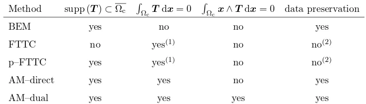
The table 1 below summarizes the main characteristics of the currently used methods to solve the TFM problem.
Method supp (T)⊂Ωc RΩcTdx= 0
R
Ωcx∧Tdx= 0 data preservation
BEM yes no no yes
FTTC no yes(1) no no(2)
p–FTTC yes yes(1) no no(2)
AM–direct yes yes no yes
AM–dual yes yes yes yes
Table 1. Main characteristics of the current methods for solving the TFM problem. The p–FTTC method is introduced in section 4.4. AM–direct is the adjoint method presented in section 3 and defined by constrained space (24) and the equations (26) and (27). AM–dual is the adjoint method described in [25]. (1) The FTTC and p–FTTC methods impose only that R
supp(T)Tdx= 0 and
(2) use interpolated data.
Conditions of use and limits of applicability. Two limits of applicability of the FTTC method exist. The first one concerns the validity of the formulation and the second one is related to the accuracy of the numerical DFT.
The validity of the formulation used to define the direct problem (28) is equivalent to that of the expression (29) of the Green tensor. Hence, it is equivalent to the possibility to approximate the 3D gel domain by a half-plane.
The accuracy which we are discussing here is not the accuracy of the quadrature formula used to approximate the Fourier coefficients (30) but the capacity of the DFT to avoid the overlap of the translated spectrafcnduring summation (32). It only concerns the (interpolated) beads displacements since the exact Fourier transform of the Green tensor is available thanks to (35). As indicated in section 4.2, the conditions (34) are sufficient to achieve this kind of accuracy. If these conditions are not satisfied, then the computed Fourier transform of the beads displacements is a poor approximation. In the context of inverse problems, this loss of accuracy can be dramatic. To avoid these difficulties, it is sufficient to choose a spatial step size hk small enough in order to satisfy condition (34b).
4.4.
The projected FTTC method (p–FTTC)
method coupled with a Tikhonov regularization and ends by a projection step which ensures the localization condition.
Interpolation operator. As exposed in section 4.2, the DFT (i) requires to discretize the computational domain using an uniform and structured grid, and (ii) the knowledge of the beads displacement at every node in this grid. The role of the interpolation step is to estimate these new displacements, denoted by ug, from the knowlegde of the experimental displacements ub. This estimation is performed by using an interpolation operator which is a linear operator from R2Nb (N
b denoting the number of beads) into a specific functional space depending on the regularity imposed to the interpolant.
We used the natural neighbor interpolation (see [5] for a review of the main methods for solving the scattered data interpolation problem). This method gives a good balance between accuracy and computational time. The interpolant function ug can be written as the linear combination
ug : x∈Ω7−→ug(x) =
Nb
X
k=1
ϕk(x)ub,k∈R2 (36)
where ϕk(·) is the shape function associated with thek-th bead displacementub,k. The shape functions have a compact support and are globallyC0[23] (and evenC∞except at beads locations). In the sequel, we denote
byXg the space of all functions of the form (36).
Tikhonov regularization of the unconstrained FTTC method. Schwarz et al. pointed out [22] that the TFM problem cannot be correctly solved with the BEM without using a regularization method. This observation was confirmed for the FTTC method [21]. Here, we derive a Tikhonov regularized FTTC method by using the framework developed in section 2.
The spaces are chosen as follows. Since we want to replace the dataubby its interpolant ug defined by (36), the spaceXb must be replaced byXg. So, we chooseV =Xg. On the other hand, we chooseH =L2(Ω). We do not impose any biomechanical constraint, soHc =H. Note that sinceXb=Xgis then a finite dimensional space, we can simultaneously identifyH andXbwith their respective dual spaces.
Under these conditions, both operatorsPc and B involved in (17) reduce to the identity operator. Then, we can rewrite the abstract equations (17) as the equation A−TA−1T
ε+εTε = A−Tub. Taking into account the expression (28) of the operator A, this equation becomes GT∗G∗T
ε+εTε = GT∗ub in the physical space and, thanks to the identity (31),
b
GT(ξ)Gb(ξ)Tcε(ξ) + εTcε(ξ) = GbT(ξ)ucb(ξ) for ξ∈R2 (37)
in the Fourier space. This last equation appears as a regularized form of the normal equation related to b
G(ξ)Tcε(ξ) =ucb(ξ).
The p–FTTC method. The p–FTTC method improves the classical FTTC method by allowing to impose the localization constraint with a projection operator. It can be summarized as follows.
(1) Compute the interpolant ug ∈Xg of the experimental beads displacements ug in the physical space and approximate its Fourier transformucg using the DFT.
(2) For each ξn 6= 0 describing the non-zero nodes of the discretization grid (33) in the Fourier space, computeTcε(ξn) by solving equation (37) for ξ=ξn.
(3) Impose the zero total force constraintRΩTεdx= 0 (over Ω, not over the cell domain Ωc) in the Fourier space by settingTcε(0) = 0.
(5) Finally, impose the localization constraint supp (Tε) ⊂ Ωc by applying the projection operator Pcs defined byPcsT : x∈Ω7−→(PcsT) (x) =χc(x)T(x) ∈ R2.
Note that the traction stressTε calculated by the previous algorithm does not belong to the spaceHc defined in (24). In other words,Tεsatisfies the localization constraint (supp (T)⊂Ωc) but, in general,RΩcTεdx6= 0.
5.
Numerical comparison of Adjoint and p–FTTC methods
In this last section, results from simulations obtained using the adjoint method and the p–FTTC method are discussed. A particular attention is paid to the choice of the regularization parameter.
Experimental data. Experiments involving GFP–transfected RT112 cells (from bladder epithelial tissues, rather low invasiveness degree) have been performed on Polyacrylamide gels with Young modulus E= 10 kPa and Poisson ratio ν = 1/2. Measurements of fluorescent beads positions have been made using confocal mi-croscopy and displacements were deduced using a technique previously described [3].
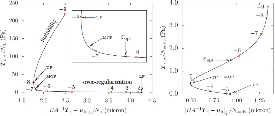
L–curve. There exists several methods [14, 16, 26] to select a suitable value of the regularization parameter ε. This choice is a crucial step to yield an accurate approximation of the stress field. In order to avoid the use of any additional information (for example, error level in experimental data), we have chosen theL–curve criterion [15]. This method is based on a plot of the parametric curve of the stress norm |Tε|2 versus the residual normBA−1T
ε−ub2 for all ε > 0 (|v|2 denoting the euclidian norm of a discretization of v). The L–curves constructed by the adjoint and p–FTTC methods can be seen in Fig. 5 below (in unusual linear scale).
The L–curve depicts the influence of the regularization parameter on the stress field. The one obtained with the adjoint method can be interpreted as follows. Low values of εlead to high values of |Tε|2. Indeed, when εtends to zero the regularization term vanishes in the Tikhonov functional (6) and then the stress fieldTε is strongly affected by the excitation of experimental errors in data. Next, the stability increases with the value of εand the L–curve is decomposed into three regions. In the first one, |Tε|2 and
BA−1T
ε−ub
2 decreases simultaneously until a turning point is reached. In the second region, just after this turning point, only |Tε|2 decreases whileBA−1T
ε−ub2 increases reasonably. In this region, the curvature is high and the point where the curvature is maximal is the corner of the L–curve. The third region is characterized by a low value of the curvature. In this region, |Tε|2 decreases slowly and
BA−1T
ε−ub2 increases steadily. This is due to the importance of the regularization term in the Tikhonov functional. Hence, in this region, the stress field is over-regularized. Finally, for high values ofεthe Tikhonov functional is totally dominated by its regularization term, so |Tε|2 tends to zero and the residual norm tends to|ub|2. Hence, the L–curve presents a limit point whenεtends to infinity.
The L–curve obtained with the p–FTTC method is somehow different, but turning point and its corner are even more evident, so that the regions identified in the previousL–curve can be identified.
Selection of the regularization parameters. In the region of higher curvature, the requirements of stability forTε and of the small value for the residual norm are well balanced. So, the value ofεcorresponding to the corner of theL–curve is a natural candidate to give the optimal value of the regularization parameter [15]. We have checked this value, but, unfortunately, the corresponding stress field was unrealistic.
To find a better estimate of the stresses, we have used the following technique. We have visualized the stress vectors corresponding to a range of values ofεnear to the corner of theL–curve. Initially, the stress vectors point in all directions, with a very irregular manner, then asεis increased, a rearrangement of the vectors orientation takes place and these stresses directions become stable. Asε is further increased, the vector patterns remain stable in direction but their norms decrease. This last behavior corresponds to over-regularized solutions. Thus the optimum value of ε is chosen as the first value leading to a stabilized orientation for the directions of the stress vectors. This chosen value is found in the vicinity of the high curvature of the curve, but not necessarily at the highest local curvature. With the data and parameters used in Fig. 5, we have obtainedε= 7.0×10⁻⁶ in the case of the adjoint method andε= 1.5×10⁻⁶ in the case of the p–FTTC method.
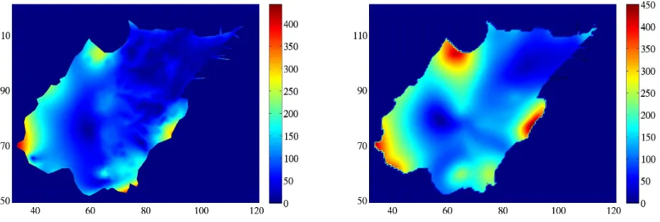
Comparison of the computed traction stresses. The estimated stress fields corresponding to these selected values ofεcan be seen in Fig. 4 (stress vectors) and 5 (stress norm) below. These results seem in good agreement. But although the orders of magnitude are rather similar, some differences are however present. In particular (i) the areas of the high stresses are different, (ii) different stress directions are found in the lower right and top parts of the cell. Moreover, as shown in Fig. 6, the adjoint method predicts non negligible stresses in filipodia (sharp shapes of the cell membrane) while the p–FTTC method does not that. Finally, the p–FTTC smoothes the stresses more than the adjoint method.
Conclusion. It can be concluded that the p–FTTC can be a good approximation of the solution but it has disadvantages as compared to the AM method. The p–FTTC method is in any case more accurate than the classical FTTC method [8], which does not ensure the biomechanical constraints of zero stresses outside the cell. Furthermore, the second condition (null sum of stresses) is also satisfied. As one wants to improve this solution, it is better to use the AM method, in particular it enables to obtain local refinements of the solution in particular where filipodia are located. It is important to define stress directions precisely at these locations, whereas the p–FTTC method does not provide this information at all.
6.
Conclusion
40 60 80 100 120 50
70 90 110
400 Pa
40 60 80 100 120
50 70 90 110
400 Pa
Figure 4. Stresses vectors obtained with the adjoint method (left) and the p–FTTC metod (right). The parameters have the same values as in Fig. 5. Regularizatioin parameter: ε = 7×10⁻⁷ for the adjoint method andε= 1.5×10⁻⁶ for the p–FTTC method.
Figure 5. Stresses norms obtained with the adjoint method (left) and the p–FTTC metod (right). The parameters have the same values as in Fig. 4.
satisfied by the cell are related to mathematical constraints and are imposed thanks to a projection operator. As specific applications, the adjoint and the FTTC methods can be derived in this framework by choosing suitable formulations for the direct problem. Furthermore, we have used the projection operator of the adjoint method to improve the FTTC method. This improvement imposes the zero traction stress condition outside the cell and it is achieved using the regularized FTTC method followed by a projection step. This improved FTTC, the so-called p–FTTC, yields acceptable results.
104 106 108 110 112 100
102 104
100 Pa
104 106 108 110 112
100 102 104
200 Pa
Figure 6. Stress field near a filipod obtained with the adjoint method (left) and the p–FTTC method (right). The parameters have the same values as in Fig. 5.
References
[1] R. A. Adams and J. J.-F. Fournier.Sobolev Spaces, volume 140 ofPure and applied mathematics. Academic Press, New York, USA, 2003.
[2] D. Ambrosi. Cellular traction as an inverse problem.SIAM J. Appl. Math., 66:2049–2060, 2006.
[3] D. Ambrosi, A. Duperray, V. Peschetola, and C. Verdier. Traction patterns of tumor cells.J. Math. Biol., 58:163–181, 2009. [4] N. Q. Balaban, U. S. Schwarz, D. Riveline, P. Goichberg, G. Tzur, I. Sabanay, D. Mahalu, S. Safran, A. Bershadsky, L. Addadi,
and B. Geiger. Force and focal adhesion assembly: a close relationship studied using elastic micropatterned substrates.Nat. Cell Biol., 3(5):466–472, 2001.
[5] T. Bobach.Natural Neighbor Interpolation - Critical Assessment and New Results. PhD thesis, TU Kaiserslautern, 2008. [6] A. B¨ottcher, B. Hofmann, U. Tautenhahn, and M. Yamamoto. Convergence rates for Tikhonov regularization from different
kinds of smoothness conditions.Applicable Analysis, 85(5):555–578, 2006.
[7] H. Brezis.Functional Analysis, Sobolev Spaces and Partial Differential Equations. Universitext. Springer verlag, New York, 2011.
[8] J. P. Butler, I. M. Tolic-Norrelykke, B. Fabry, and J. J. Fredberg. Traction fields, moments, and strain energy that cells exert on their surroundings.Am. J. Physiol. Cell Physiol., 282(3):C595–C605, 2002.
[9] P. G. Ciarlet.Mathematical elasticity: Volume 1 Three-Dimensional Elasticity, volume 20 ofStudies in Mathematics and its Applications. North-Holland, Amsterdam, 1988.
[10] P. G. Ciarlet.Introduction to linear numerical algebra and optimization. Texts in Applied Mathematics. Cambridge University Press, Cambridge, 1989.
[11] M. Dembo and Y. L. Wang. Stresses at the cell-to-substrate interface during locomotion of fibroblasts.Biophys. J., 76(4):2307– 2316, 1999.
[12] H. W. Engl, M. Hanke, and Neubauer N.Regularization of Inverse Problems, volume 375 ofMathematics and its applications. Kluwer Academic Publishers, Dardrecht, The Netherlands, 1996.
[13] M. Frigo and S. G. Johnson. The design and implementation of FFTW3.Proceedings of the IEEE, 93(2):216–231, 2005. Special issue on “Program Generation, Optimization, and Platform Adaptation”.
[14] P. C. Hansen.Discrete Inverse Problems: Insight and Algorithms. Fundamentals of Algorithms. SIAM Press, Philadelphia, PA, USA, 2010.
[15] P. C. Hansen and D. P. O’Leary. The use of the l-curve in the regularization of discrete ill-posed problems. SIAM J. Sci. Comput., 14(6):1487–1503, 1993.
[17] L. Landau and E. Lisfchitz.Th´eorie de l’´elasticit´e. Editions Mir, 1967.
[18] J. L. Lions.Optimal control of systems governed by partial differential equations. Springer verlag, Berlin, 1971.
[19] R. Michel, V. Peschetola, B. Bedessem, J. Etienne, D. Ambrosi, A. Duperray, and C. Verdier. Inverse problems for the determination of traction forces by cells on a substrate: a comparison of two methods.Comput Methods Biomech. Biomed. Eng., 15(S1):27–29, 2012.
[20] V. Peschetola, V. Laurent, A. Duperray, R. Michel, D. Ambrosi, L. Preziosi, and C. Verdier. Time–dependent traction force microscopy for cancer cells as a measure of invasiveness.Cytoskeleton, 70(4):201–214, 2013.
[21] B. Sabass, M. L. Gardel, C. M. Waterman, and U. S. Schwarz. High resolution traction force microscopy based on experimental and computational advances.Biophys. J., 94(1):207–220, 2008.
[22] U. S. Schwarz, N. Q. Balaban, D. Riveline, A. Bershadsky, B. Geiger, and S. A. Safran. Calculation of forces at focal adhesions from elastic substrate data: the effect of localized force and the need for regularization.Biophys. J., 83(3):1380–1394, 2002. [23] N. Sukumar, B. Moran, A. Yu. Semenov, and Belikovm V. V. Natural neighbour galerkin methods.Int. J. for Num. meth.
Engineering, 50(1):1–27, 2001.
[24] H. Tanimoto and M. Sano. Dynamics of traction stress field during cell division.Phys. Rev. Lett., 109:248110, 2012.
[25] G. Vitale, D. Ambrosi, and L. Preziosi. Force traction microscopy: an inverse problem with pointwise observations.J. Math. Anal. Appl., 395(2):788–801, 2012.
[26] C. R. Vogel.Computational methods for inverse problems. Frontiers in Applied Mathematics. SIAM Press, Philadelphia, PA, USA, 2002.