Wavelet­ based image denoising based on a mixture of laplace distributions

© Shiraz University

WAVELET BASED IMAGE DENOISING BASED ON

A MIXTURE OF LAPLACE DISTRIBUTIONS

H. RABBANI AND M. VAFADOOST

Dept. of Biomedical Engineering, Amirkabir University of Technology, Tehran I. R. of Iran Email: [email protected]

Abstract– The performance of various estimators, such as maximum a posteriori (MAP), strongly depends on correctness of the proposed model for distribution of noise-free data. Therefore, the selection of a proper model for the distribution of wavelet coefficients is very important in wavelet based image denoising. This paper presents a new image denoising algorithm based on the modeling of wavelet coefficients in each subband with a mixture of Laplace random variables. Indeed, we design a MAP estimator which relies on mixture distributions. Using this relatively new statistical model we are better able to capture the heavy-tailed nature of wavelet coefficients. The simulation results show that our proposed technique achieves better performance than several published methods, both visually and in terms of root mean squared error (RMSE).

Keywords– MAP estimator, mixture model, wavelet transforms

1. INTRODUCTION

Usually, noise reduction—the process of noise-free data estimation from noisy data observation—is an essential part of many image processing systems (Fig. 1). The main sources of noise arise from the imaging devices during image formation and channels during transmission [1]. A suitable noise reduction algorithm is used to reconstruct the main information of the image, so that the obtained image will have the greatest peak signal-to-noise ratio (PSNR) and least visual artifacts [1]. In recent years there has been a fair amount of research on wavelet-based image de-noising [2-8]. The motivation of denoising in the wavelet domain is that, while the wavelet transform is good at energy compaction, the small coefficients are more likely caused by noise, and the large coefficients caused by important signal features [5]. The small coefficients can be thresholded without affecting the significant features of the image [3]. Thresholding is a simple non-linear technique, which usually operates on one wavelet coefficient at a time [2]. In its most basic form, each coefficient is thresholded by comparing against the threshold: if the coefficient is smaller than the threshold, set to zero; otherwise it is kept or modified. Replacing the small noisy coefficients by zero and applying the inverse wavelet transform on the result may lead to reconstruction with the essential signal characteristics and with less noise [3].

Many of the wavelet based denoising algorithms have been developed based on soft thresholding proposed by Donoho [2], and examples of alternative approaches can be found in [5-11]. Generally, these methods lead to a threshold value that must be estimated correctly in order to obtain a good performance. Early methods, such as VisuShrink [3] use a universal threshold, while more recent ones, such as SureShrink [4] are subband adaptive algorithms and have better performance. BayesShrink [5], which is also a data-driven subband adaptive technique, outperforms both Visu-Shrink and SureShrink.

Fig. 1. Image processing chain [1]

The problem of wavelet based image denoising can be expressed as an estimation of clean coefficients from noisy data with Bayesian estimation techniques. If the MAP estimator is used for this problem, the solution requires a priori knowledge about the distribution of wavelet coefficients. Based on the distribution type, the corresponding estimator (shrinkage function) is obtained.

Various probability density functions (pdfs) such as Gaussian, Laplace, generalized Gaussian or other distributions were proposed for modeling noise-free wavelet coefficients [11-12]. For example, the classical soft threshold shrinkage function can be obtained by a Laplacian assumption. Bayesian methods for image denoising using other distributions have also been proposed [13-17].

In this paper we use a mixture of Laplace random variables to model the wavelet coefficients in each subband. Because the energy compactness property of the wavelet makes it reasonable to assume that essentially, only a few large coefficients contain information about the underlying image, the marginal distribution of wavelet coefficients is highly kurtoutic, and can be described using suitable long-tailed distributions [11]. In [18], the wavelet-based hidden Markov model (HMM) is proposed for statistical signal processing and a mixture of Gaussian distributions is used for modeling this heavy-tailed property of wavelet coefficients. Our approach is similar to the method reported in [18], but we use Laplace components instead of Gaussian components. Because Laplace pdf has a large peak at zero and its tails fall significantly slower than a Gaussian pdf of the same variance, a mixture of Laplace pdfs can improve the modeling of wavelet coefficients distribution.

2. BAYESIAN DENOISING

In this section, the denoising of an image corrupted by white Gaussian noise will be considered. We observe a noisy signal g=x+n where n is independent, white, zero-mean Gaussian noise and we wish to estimate the noise-free signal x as accurately as possible according to some criteria [3]. In the wavelet domain, if we use an orthogonal wavelet transform, the problem can be formulated as y=w+n, where y is the noisy wavelet coefficient, w is the noise-free wavelet coefficient, and n is noise, which is independent white zero mean Gaussian [3].

If p_W(w) denotes pdf of random variable W for W =w and pW|Y(w|y) denotes the conditional pdf of random variable W for W =w when given random variable Yfor Y =y, the MAP estimator below will be used to estimate w from the noisy observation y [5]. This estimator is defined as

y) | (w p argmax (y)

wˆ _w|y w

= (1)

Using Bayesian rule [5] we get

(y) p (w) p w) | (y p y) | (w p y w w | y y | w =

Therefore, one gets

(y) p (w) p w) | (y p argmax (y) wˆ y w w | y w =

Because the term py(y) does not depend on w, the value of w that maximizes the right hand side is not influenced by the denominator. Therefore the MAP estimate of w is given by

(w)] p w) | (y [p argmax (y)

wˆ _{y|w w}

w =

Because y is the sum of w and n, a zero-mean Gaussian pdf, when w is a known constant, y will be a Gaussian pdf with mean w. Therefore, if the pdf of n is p_n(n), then py|w(y|w) will be pn(y−w).

Thus, Eq. (1) can be written as

(w)] p w). (y [p argmax (y)

wˆ _{n w}

w

−

= (2)

Equation (2) is also equivalent to

f(w)] w)) (y [log(p argmax (y)

wˆ _n

w

+ −

= (3)

where f(w)=log(pw(w)).

We have assumed the noise is zero mean Gaussian with variance σ_n,

) exp( . : ) , ( ) ( ₂ n 2 n n n 2 n 2 1 n Gaussian n p σ − π σ = σ

= (4)

Replacing (4) in (3) yields

)] ( 2 ) ( [ max arg ) (

ˆ y y w₂ 2 f w

w n w + − − = σ

Therefore we can obtain the MAP estimate of w by setting the derivative with respect to wˆ equal to zero. That gives the following equation to solve for wˆ .

For example, if p_w(w) is assumed to be Gaussian(w,σ), then f(w)=−log( 2πσ)−w2/2σ2, and the estimator can be written as

y σ σ σ (y) wˆ 2 n 2 2 +

= (6)

a) Soft thresholding

We now need to model p_w(w) for the distribution of wavelet coefficients. The pdf for wavelet coefficients

) (w

pw is often modeled as a generalized (heavy-tailed) Gaussian [7],

) s w exp( q). K(s, (w) p q

w = − (7)

where s,q are the parameters for this model, and K(s,q) is the normalization constant (which depends on

sand q). Other pdf models have also been proposed [7-17]. Substitution of q=1 in (7) simplifies the equation to a Laplace pdf,

) w σ 2 exp( 2 σ 1 : σ) Laplace(w, (w)

p_w = = − (8)

In this case

w w

f( ) log( 2) 2. σ σ − − = and so ) ( . 2 )

(w sign w f σ − = ′ therefore ) ˆ ( . 2

ˆ 2 sign w

w y n σ σ + = thus ⎪ ⎩ ⎪ ⎨ ⎧ < − < ≤ − < + = y T T y T y T T y T y w , , 0 , ˆ where σ σ2 2 _n

T = .

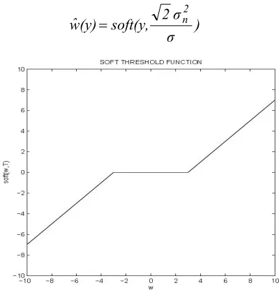
This is the soft threshold nonlinearity based on the MAP estimator. Figure 2 shows a graph of wˆ as a function of y. Other approaches give different formulas for choosing the threshold [11, 17]. The formula

is often written in the following way

+ − = ) σ σ 2 y sign(y).( (y) wˆ 2

n ₍₉₎

Here (a)₊is defined as

⎩ ⎨

⎧ < =

+ _{a otherwise}if a

a) 0 0

( Let’s define the soft operator as

+ − = ( ).( ) : ) ,

(g τ sign g g τ soft

) σ

σ 2 soft(y, (y)

wˆ

2 n

= (10)

Fig. 2. Shrinkage function corresponding to the Laplace pdf (soft threshold)

The main idea in soft thresholding is to subtract the threshold value T from all coefficients larger than T and to set all other coefficients to zero. The threshold T = 2σ_n2/σ has an intuitive appeal. The normalized threshold, T/σn= 2σn/σ, is inversely proportional to σ , the standard deviation of w, and proportional to σ_n, the noise standard deviation. When σ_n/σ<<1, the signal is much stronger than the noise. Therefore T/σ_n is chosen to be small in order to preserve most of the signal and remove some of the noise. Vice versa, when σ_n/σ >>1, the noise dominates. In this case, the normalized threshold is chosen to be large to remove the noise, which has overwhelmed the signal. Thus, this threshold is adapted to both the signal and noise characteristics, which are reflected in parameters σ_n and σ [5].

1. Parameters estimation: To apply the soft threshold rule we need to know σn and σ . Experiments

show that σ is quite different from scale to scale. Figure 3 shows the standard deviation of each wavelet

subband for the Lena image. Thus, we must estimate a different σ for each subband only from the noisy

data. In fact, the results lead to a subband-dependent threshold.

Because the wavelet coefficients of the noise free image and the noise are independent, we have

VAR[n] VAR[w]

VAR[y]= +

in which VAR[x] is variance of the random variable x.

As we assume that the variance of the noise is known, we write

2

2 _{[ ]}

n

y

VAR σ

σ = −

The variance of y can be computed from each subband using the standard formula [3], where we assume all quantities are zero mean,

] [ ]

[y MEAN y2

VAR =

where MEAN[x] is the empirical mean [3] of x. So we estimate σ as

2 n 2_{] σ} MEAN[y

σˆ = −

In case we have a negative value under the square root (it is possible because these are estimates) we can use

,0) σ ] max(MEAN[y

σˆ = 2 − _n2 (11)

When σ_n is unknown, to estimate the noise variance from the noisy wavelet coefficients, a robust median estimator is used from the finest scale wavelet coefficients [3].

scale finest in

HH subband y

6745 0

y median

i

i 2

n

∈ =

σ ,

.

) (

(12)

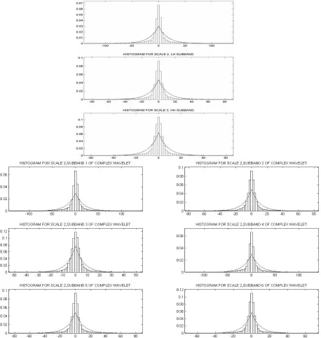
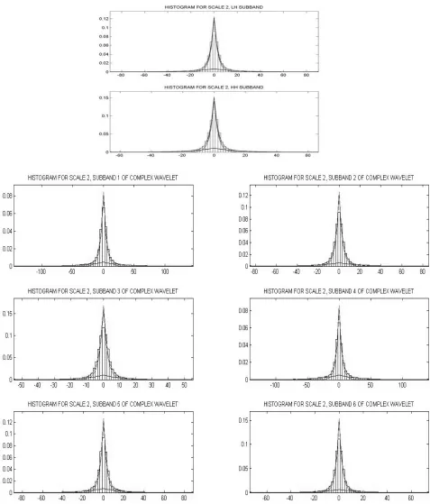
2. Modeling wavelet coefficients as a single Laplace distribution: In this section, a single Laplace pdf is used to model a histogram of a 512×512 Lena image in each subband. Figure 4 illustrates the

histograms of the wavelet coefficients in the second scale and the best Laplace pdf is fitted to these

histograms.

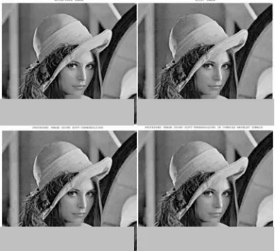
We use soft thresholding for noise reduction of the 512×512 Lena image. Zero mean white Gaussian noise is added to the original image (σ_n=10). The RMSE between the original image and the processed image in a standard wavelet domain is calculated to be 4.97. The RMSE between the original image and the noisy image is simply σn, the standard deviation of the noise, for this example is set at 10. Therefore, the wavelet domain soft thresholding reduced this noise level by more than a factor of 2. Figure 5 shows a break down of the square error in each subband. Because a few large coefficients which correspond to coarser scales represent the main features of the signal, noise mostly affects small coefficients corresponding to the finer scales. Therefore, we can see in this figure that most of the square error occurs in the finer scales. The original image, the noisy image and the denoised image produced using the soft threshold, are illustrated in Fig. 6.

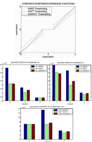
Due to the effectiveness and simplicity of soft thresholding, it is frequently used in the literature, but other shrinkage functions have also been proposed [13-17]. For example, Fig. 7 shows the differences between soft thresholding, hard thresholding [2-4] and garrot thresholding [8].

Although soft thresholding usually has acceptable results for denoising, it does not have a good performance for other kinds of noise such as Poisson, which is signal-dependent. In this case, algorithms that use local variances have better results [17, 19].

Fig. 4. Histograms of the wavelet coefficients and the best fitted Laplace model in second scale of Lena image

b) Denoising based on mixture models

A mixture model for a random variable has a pdf that is the sum of two simpler pdfs,

(w) p a) (1 (w) ap

p(w)= ₁ + − ₂ (13)

matching the histogram of a given dataset. If there are too many parameters, then it will be difficult to

estimate those parameters accurately from the data. There is a trade off between the number of parameters

and the ability to estimate them.

In the following sections we will use a mixture of two Laplace pdfs:

) w σ

2 exp( 2 σ

1 a) (1 ) w σ

2 exp( 2 σ

1 a

) σ Laplace(w, a).

(1 ) σ Laplace(w, .

a (w) p

2 2

1 1

2 1

w

− −

+ −

=

− + =

(14)

to model the distribution of wavelet coefficients of images. It will be necessary to estimate the three parameters σ1,σ2 and a from the data. While σ1 and σ2 represent the standard deviation of the individual components, they are not very easily related to the standard deviation of the random variablew, for example

2 2 2 2

1

2 _{(1 )}

]

[w a σ a σ

VAR ≠ + −

Nor are other simple relations available. The estimation of the three parameters is more difficult than it is

for a single component model. For a mixture model, an iterative numerical algorithm is required to estimate the parameters. The most frequently used algorithm to determine the parameters of a mixture model is the EM algorithm. A simple description of the EM algorithm can be found in the Appendix.

Fig. 5. Square error in each subband of Lena image after soft thresholding

1 2 3 0

0.5 1 1.5 2 2.5 3 3.5 4 4.5x 10

6 SQUARE ERROR IN SUBBAND HL

SCALE

HL HARD HL SOFT HL GARROT

1 2 3

0 2 4 6 8 10 12 14 16 18x 10

5 SQUARE ERROR IN SUBBAND LH

SCALE

LH HARD LH SOFT LH GARROT

1 2 3

0 2 4 6 8 10 12 14x 10

5 SQUARE ERROR IN SUBBAND HH

SCALE

HH HARD HH SOFT HH GARROT

Fig. 7. Difference between soft, hard and garrot thresholding and RMSE in each subband of Lena image after denoising with these methods

Note that the random variable w in (13) is not the result of adding two random variables. If that were the case, then p(w) would be a convolution of p₁(w) and p₂(w). Instead, w can be generated using a two step procedure. First, generate a binary random variable v according to

a v

p a v

p( =1)= , ( =2)=1−

The value of v will be either 1 or 2. For v=1, p1 is used to generate w, while for v=2, p2 is used to generate w. Because this procedure produces a random variable w with the pdf in Eq. (13), w can be considered as being generated by either p1 or by p2 (even if that is not how w is physically produced).

1. Modeling wavelet coefficients as a mixture of Laplace pdfs: In [18] a mixture of two Gaussian pdfs is proposed for modeling wavelet coefficients distribution

) σ , Gaussian(w a).

(1 ) σ , Gaussian(w .

a (w)

Because the Laplace pdf has a large peak at zero and tails that fall significantly slower than a Gaussian pdf of the same variance, a mixture of Laplace pdfs can improve the modeling of wavelet coefficients distribution.

In this section, a mixture of two Laplace distributions is used to model the wavelet coefficients of a 512

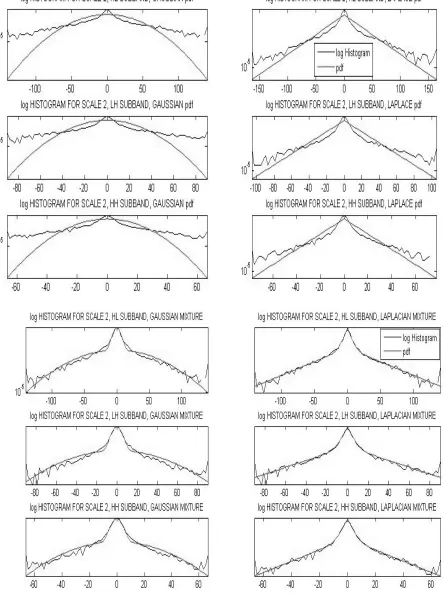
512× Lena image in each subband. Figure 8 shows the mixture pdf obtained using the EM algorithm, together with the histogram for the second scale. We see that the mixture of two Laplace pdfs follows the histogram much more closely than both the Gaussian mixture model and a single Laplace pdf (Fig. 9).

The nonlinear soft threshold rule for wavelet-based image denoising is the MAP estimator of the coefficients in Gaussian noise when the noise free coefficients are distributed according to the Laplace distribution. However, the plots in this section show that the Laplace distribution is not always an accurate model for the distribution of the noise-free coefficients, therefore, an alternative non-linearity derived using the mixture model may work more effectively than the soft threshold rule. In the next section we will illustrate the nonlinear shrinkage rule derived from the Laplacian mixture model, and later compare its performance with the soft threshold rule.

2. Threshold functions derived from the mixture models: This section describes a non-linear shrinkage function for wavelet-based denoising derived by assuming that noise-free wavelet coefficients follow a mixture model. Specifically, we assume that the noise-free wavelet coefficients are modeled as a mixture of two Laplace random variables.

If w follows the mixture pdf,p(w)=ap₁(w)+bp₂(w) where a+b=1 and p₁ and p₂ are valid pdfs individually, then how can we estimate w from a noisy observation y=w+n, where n is an independent zero-mean Gaussian random variable with standard deviation σ_n? Because the estimate of w depends on

y, it is denoted bywˆ(y).

One way to obtain an estimate is by the following rule:

(y) wˆ (y) p (y) wˆ (y) p (y)

wˆ = _{a 1} + _{b 2} (16)

where pa(y) is the probability that w was generated by p1, and where similarly, pb(y) is the probability that w was generated by p2. The expression wˆ1(y) is an estimate of w based on the assumption that w was generated by p1, and that similarly wˆ2(y) is an estimate of w based on the assumption that w was generated by p2. If p1 and p2 are Laplace pdfs with parameters σ1 and σ2 respectively, then the soft threshold function can be used to get wˆ₁(y) and wˆ₂(y). We would have

) 2 , ( ) ( ) 2 , ( ) ( ) ( ˆ

2 2

1 2

σ σ σ

σ _n

b n

a ysoft y p ysoft y

p y

w = + ,

but we still need to determine pa(y) and pb(y). For these values we can use the formulas based on Bayes

theorem [5] as follows:

(y) bg (y) ag

(y) ag (y)

p

2 1

1

a = ₊ (17)

(y) bg (y) ag

(y) bg (y)

p

2 1

2

b = ₊ (18)

where g1(y) is the pdf of y under the assumption that w was generated by p1, and similarly, g2(y) is

) σ σ 2 soft(y, (y) bg (y) ag (y) bg ) σ σ 2 soft(y, (y) bg (y) ag (y) ag (y) wˆ 2 2 n 2 1 2 1 2 n 2 1 1 + + + = (19)

Because y is the sum of w and independent Gaussian noise, the pdf of y is the convolution of the pdf of

w and the Gaussian pdf,

) ( ) ( ) ( * ) ( ) ( * ) ( ) ( * )) ( ) ( ( ) ( 2 1 2 1 2 1 y bg y ag y p y bp y p y ap y p y bp y ap y p n n n y + = + = + =

If w follows the Laplacian mixture model, according to Eq. (14) we have

) , ( * ) , ( ) ( ₁

1 y Laplce y Gaussian y n

g = σ σ )

σ 2 y exp( . σ π 2 1 * ) y σ 2 exp( σ 2 1 2 n 2 n 1 1 − −

= (20)

and ) , ( * ) , ( ) ( ₂

2 y Laplce y Gaussian y n

g = σ σ )

σ 2 y exp( . σ π 2 1 * ) y σ 2 exp( σ 2 1 2 n 2 n 2 2 − −

= (21)

) (

1 y

g and g2(y) are not one of the standard pdfs that are commonly known. Figure 10 shows the pdf of the sum of a Laplace and a Gaussian random variable. A formula for pdf of y that is the sum of a Laplace random variable with standard deviation σ_i and a zero-mean Gaussian random variable with variance σ_n is given by [20]

2 , 1 , )] 2 ( ) 2 ( ).[ 2 exp( 2 2 1 ) ( ₂ 2 = σ + σ σ + σ − σ σ σ − σ = i y erfcx y erfcx y y g n i n n i n n i i (22) where

∫

If we use the notation LapGauss(y,σ_x,σ_n) for the pdf in (22), then we will have

) , , ( : ) ( ) , , ( : ) ( 2 2 1 1 n n y LapGauss y g y LapGauss y g σ σ = σ σ =

and so

y

Fig. 9. Histograms of the wavelet coefficients and the best fitted pdf in second scale of Lena image in the log domain. From top left, clockwise: Gaussian pdf, Laplace pdf, a mixture of

Fig. 10. pdf of the sum of a Laplace and a Gaussian random variable

Figure 11 shows the histogram of the noise-free 512×512 Lena image and the mixture of two Laplace pdfs fitted to it, as well as the histogram of the noisy image corrupted with additive Gaussian noise with

10

=

n

σ and the mixture of two LapGauss pdfs fitted to it.

To find the shrinkage function, the LapGauss pdf is not needed directly, but only as it appears in the following expression = + = ) ( ) ( ) ( ) ( 2 1 1 y bg y ag y ag y p_a ) , , ( ) , , ( ) , , ( 2 1 1 n n n y bLapGauss y aLapGauss y aLapGauss σ σ σ σ σ σ +

After canceling some common terms and rearranging we get

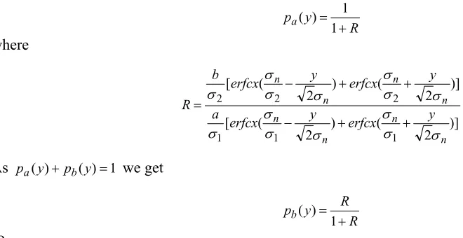
R y p_a + = 1 1 ) ( where )] 2 ( ) 2 ( [ )] 2 ( ) 2 ( [ 1 1 1 2 2 2 n n n n n n n n y erfcx y erfcx a y erfcx y erfcx b R σ σ σ σ σ σ σ σ σ σ σ σ σ σ + + − + + − =

As pa(y)+pb(y)=1 we get

R R y pb = ₊

1 ) (

) 2 , ( 1

) 2 , ( 1

1 ) ( ˆ

2 2

1 2

σ σ +

+ σ

σ +

= n _{soft y} n

R R y

soft R y

w (24)

where R is given by the formula above.

Fig. 11. Histogram of the noise-free and noisy Lena image and the best fitted mixture model

Like the soft threshold function, this nonlinear shrinkage function that we call LapMixShrink reduces (or shrinks) the value of y to estimate w. For several different values of the model parameters, some of the shrinkage functions are given in Fig. 12. The nonlinear function does not shrink large values of

y

mixture of two LapGauss components, and assuming the noise variance σ_n is known, we can estimate the model parameters a,σ₁ and σ2 using the EM algorithm. The threshold functions for each subband of the

512

512× Lena image corrupted with additive Gaussian noise with σ_n=10 after estimating parameters is illustrated in Fig. 13.

Fig. 12. LapMixShrink function produced from a mixture of two Laplace pdf

Instead of LapMixShrik, other nonlinear shrinkage functions can be found with other mixture models. For example, if w follows the Gaussian mixture model (15), p₁ and p₂ are Gaussian pdfs with parameters σ1 and σ2 respectively. Therefore, Eq. (6) can be used to get wˆ1(y) and wˆ2(y) in Eq. (16),

y y w n2 2 1 2 1 1( )

ˆ

σ σ

σ +

= , w y y

n2

2 2

2 2 2( )

ˆ σ σ σ + =

In this case, g₁(y) and g₂(y) in Eqs. (17) and (18) can be written as

) , ( ) , ( * ) , ( ) ( ) , ( ) , ( * ) , ( ) ( 2 2 2 2 2 2 2 1 1 1 n n n n y Gaussian y Gaussian y Gaussian y g y Gaussian y Gaussian y Gaussian y g σ σ σ σ σ σ σ σ + = = + = =

Thus, Eqs. (17) and (18) can be written as

) , ( ) , ( ) , ( ) ( 2 2 2 2 2 1 2 2 1 n n n a y bGaussian y aGaussian y aGaussian y p σ σ σ σ σ σ + + + + = ) , ( ) , ( ) , ( ) ( 2 2 2 2 2 1 2 2 2 n n n b y bGaussian y aGaussian y bGaussian y p σ σ σ σ σ σ + + + + =

Therefore, we can write Eq. (16) as

) , ( ) , ( ) , ( ) , ( ) , ( ) , ( ) ( ˆ 2 2 2 2 2 1 2 2 2 2 2 2 2 2 2 2 2 2 2 1 2 2 1 2 1 2 2 1 n n n n n n n n y bGaussian y aGaussian y y bGaussian y bGaussian y aGaussian y y aGaussian y w σ + σ + σ + σ σ + σ σ σ + σ + σ + σ + σ + σ σ + σ σ σ + σ = (25)

Figure 14 shows this shrinkage function, that we have named the GaussMixShrink nonlinearity, for the same model parameters according to Fig. 13.

3. EXPERIMENTAL RESULTS

In the previous section, we have proposed a new statistical model for wavelet coefficients and obtained a MAP estimator for this model. This section presents image denoising examples to show the efficiency of this new model and compare it with other methods in the literature. We test our algorithm in a standard and complex wavelet transform domain. Complex wavelet transform is an over-complete wavelet transform featuring near shift invariance and has improved directional selectivity compared to the standard wavelet transform [16, 21].

Figure 15 shows part of the original image, noisy image and denoised image obtained using our shrinkage functions illustrated in Fig. 13. Denoised images with GaussMixShrink and LapMixShrink in a standard and complex wavelet domain are illustrated in Fig. 16. We also have compared our shrinkage function (24) with the classical soft thresholding estimator given in (10) for image denoising. The

512

Part of the denoised image using the soft threshold and the denoised image using the LapMixShrink function are illustrated in Fig .17 and the LH subband of the denoised images in third scale are shown in Fig. 18. The denoised image using the soft threshold has a RMSE of 4.97, while the denoised image obtained using our shrinkage function has a RMSE of 4.83. A comparison between the RMSE in each subband after denoising with soft thresholding and the LapMixShrink method is illustrated in Fig .19.

Fig. 14. The threshold functions GaussMixShrink for Lena image in each subband

Fig. 16. Denoising with GaussMixShrink and LapMixShrink for Lena image corrupted with additive Gaussian noise with σ_n=20

Fig. 17. Denoising with soft thresholding and LapMixShrink for Lena image corrupted additive Gaussian noise with σ_n=10

We also tested our algorithm for a mixture of two and three Laplace pdfs in a standard and complex wavelet domain using different additive Gaussian noise levels σ_n =10,20, 30 to three 512×512 grayscale images, namely, Lena, Barbara and Boat, and compared them with VisuShrink, SureShrink, BayesShrink and HMT. Performance analysis is done using the PSNR measure. The results can be seen in Table 1. Each PSNR value in the table is averaged over ten runs. In this table, the highest PSNR value is bolded and the best PSNR in the standard wavelet domain is underlined. As seen from the results, our algorithm mostly outperforms the others.

Table 1. Average PSNR values of denoised images over ten runs for different test images and noise levels of noisy, Visushrink, Sureshrink, Bayesshrink, HMT system and our Model 1 (two Laplace components

in wavelet domain), our Model 2 (three Laplace components in wavelet domain), our Model 3 (three Laplace components in complex wavelet domain)

Noisy VisuShrink SureShrink BayesShrink HMT Our model 1 Our model 2 Our model3 Lena

10

n =

σ 28.18 28.76 33.28 33.32 33.84 33.60 33.63 34.83

20

n =

σ 22.14 26.46 30.22 30.17 30.39 30.41 30.42 31.72

30

n =

σ 18.62 25.14 28.38 28.48 28.35 28.67 28.75 29.91

Boat 10

n =

σ 28.16 26.49 31.19 31.80 32.28 31.94 31.99 33.00

20

n =

σ 22.15 24.43 28.14 28.48 28.54 28.59 28.63 29.58

30

n =

σ 18.62 23.33 26.52 26.60 26.83 26.74 26.84 27.64

Barbara 10

n =

σ 28.16 24.81 30.21 30.86 31.36 31.40 31.43 33.09

20

n =

σ 22.14 22.81 25.91 27.13 27.80 27.25 27.30 28.88

30

n =

Fig. 18. Comparison between denoising with soft thresholding and LapMixShrink in scale 3, LH subband

4. CONCLUSION AND FUTURE WORKS

In this paper we use a LapMixShrink function based on a mixture of Laplace pdfs for modeling wavelet coefficients in each subband. Experiments show that our model has better visual results than other methods such as soft thresholding. In order to show the effectiveness of the new estimator, we compared the LapMixShrink method with effective techniques in the literature and we see that our denoising algorithm mostly outperforms the others. The performance of this subband-adaptive data-driven system is also demonstrated on the complex wavelet domain.

Instead of this shrinkage function, other nonlinear shrinkage functions can be used. For example, instead of using a Laplace pdf we can use generalized Gaussian distribution or, instead of using the MAP estimator for a mixture of Laplace random variables in Gaussian noise, we can use the minimum mean squared error (MMSE) estimator. These new pdfs and estimators may lead to better results. Also, instead of processing each wavelet coefficient individually, better denoising results can be achieved by processing

groups of wavelet coefficients together [11, 15-17]. Thus, if we can use a model for wavelet coefficients that not only is a mixture but is also bivariate, such as, bivariate Gaussian mixture, bivariate Laplacian mixture, Cauchy mixture or circular symmetric Laplacian mixture, the performance of the denoising algorithm will be improved. Because the state-of-the-art algorithms [17, 19] generally use local adaptive methods, using these methods in combination with the LapMixShrink function, such as LapMixShrink with local parameters, may further improve the denoising results.

Acknowledgements: The authors wish to acknowledge with grateful thanks the contributions of Professor

Ivan Selesnick.

REFERENCES

1. Lukac, R., Smolka, B., Martin, K., Plataniotis, K. N. & Venetsanopoulos, A. N. (2005).Vector Filtering for Color Imaging. IEEE Signal Processing Magazine, Special Issue on Color Image Processing, 22(1), 74-86. 2. Donoho, D. L. (1995). Denoising by soft-thresholding. IEEE Trans. Inform. Theory, 41, 613–627.

3. Donoho, D. L. & Johnstone, I. M. (1994).Ideal spatial adaptation by wavelet shrinkage. Biometrika, 81(3), 425– 455.

4. Donoho, D. L. & Johnstone, I. M.(1995). Adapting to unknown smoothness via wavelet shrinkage. J. Amer. Statist. Assoc., 90(432), 1200–1224.

5. Chang, S., Yu, B. & Vetterli, M. (2000). Adaptive wavelet thresholding for image denoising and compression.

IEEE Trans. Image Processing, 9, 1532–1546.

6. Coifman, R. & Donoho, D.(1995). Time-invariant wavelet denoising. in Wavelet and Statistics, A. Antoniadis and G. Oppenheim, Eds. New York: Springer-Verlag, 103, Lecture Notes in Statistics, 125–150.

7. Figueiredo, M. A. T. & Nowak, R. D.(2001). Wavelet-based image estimation: An empirical Bayes approach using Jeffrey’s noninformative prior. IEEE Trans. on Image Processing, 10, 1322–1331.

8. Gao, H. (1998).Wavelet shrinkage denoising using the non-negative garrot. J. Comput. Graph. Stat., 7, 469– 488.

9. Hyvarinen, A. (1999). Sparse code shrinkage: Denoising of nongaussian data by maximum likelihood estimation. Neural Comput., 11, 1739–1768.

11. Simoncelli, E. P. (1999). Bayesian denoising of visual images in the wavelet domain. Bayesian Inference in Wavelet Based Models, P. Müller and B. Vidakovic Eds. New York: Springer-Verlag,. 141, Lecture Notes in Statistics.

12. Vidakovic, B.(1999). Statistical Modeling by Wavelets,” New York: Wiley.

13. Jansen, M. (2001). Noise Reduction by Wavelet Threshold-ing. New York: Springer–Verlag, 161, Lecture Notes in Statistics.

14. Abramovich, F., Sapatinas, T. & Silverman, B. (1998). Wavelet thresholding via a Bayesian approach. J. R. Stat., 60, 725–749.

15. Sendur, L. & Selesnick, I. W. (2002). Bivariate shrinkage functions for wavelet-based denoising exploiting interscaledependency.IEEE Trans. Signal Processing, 50(11), 2744–2756.

16. Achim, A. & Kuruoglu, E. E.(2005). Image denoising using bivariate alpha-stable distributions in the complex wavelet domain. IEEE Signal Processing Lett., 12(1), 17-20.

17. Strela, V., Portilla, J. & Simoncelli, E. (2000). Image denoising using a local Gaussian scale mixture model in the wavelet domain. in Proc. SPIE 45th Annu. Meet, San Jose, CA (United States), 363-371.

18. Crouse, M. S., Nowak, R. D. & Baraniuk, R. G.(1998). Wavelet-based statistical signal processing using hidden Markov models. IEEE Trans. Signal Processing, 46(4), 886-902.

19. Mihcak, M. K., Kozintsev, I., Ramchandran, K. & Moulin, P. (1999). Low complexity image denoising based on statistical modeling of wavelet coefficients.IEEE Signal Processing Lett., 6, 300–303.

20. Hansen, M. & Yu, B.(2000). Wavelet Thresholding via MDL for Natural Images. IEEE Trans. Inform. Theory, 46(5).

21. Abdelnour, A. F. & Selesnick, I. W. (2001). Nearly symmetric orthogonal wavelet bases. In Proc. IEEE Int. Conf. Acoust., Speech, Signal Processing (ICASSP), Salt Lake City (United States), 3693-3696.

APPENDIX

EM algorithm:

The Expectation-Maximization algorithm is an iterative numerical algorithm that can be used to estimate the parameters of a mixture model. Each iteration consists of an E-step and an M-step. Here we give only a simple description of the EM algorithm. The mixture model is

) ( ) ( )

(x ap1 x bp2 x

p = +

where a+b=1. The data is x_n for n=1,2,...N. From the data we want to estimate the 3 parameters a,σ₁ and σ2.

The EM algorithm works by introducing an auxiliary variable that represents, for each data point, how likely that the data point was produced by one or the other of the two components p1(x) and p2(x). This

auxiliary variable is denoted by r₁(n) and r₂(n). r₁(n) represents how responsible p₁(x) is for generating data point xn, while r2(n) represents how responsible p2(x) is for generating data point xn.

The EM algorithm starts by initializing a,b,σ₁ and σ₂, and then proceeds with a sequence of E-M steps until the parameters satisfy some convergence condition. The initial values for a and b should satisfy

1

= +b

a .

The E-step calculates the responsibility factors

) ( ) (

) ( )

(

2 1

1 1

n n

n

x bp x ap

x ap n

r

+ ←

) ( ) (

) ( )

(

2 1

2 2

n n

n

x bp x ap

x bp n

r

Note that the responsibility factors are between 0 and 1 and that r₁(n)+r₂(n)=1.

The M-step updates the parameters a,b,σ1 and σ2. The mixture parameters a and b are computed by

∑

∑

1( ), 1 ( )

1

It is easy to verify that a+b=1 is guaranteed. One way to update σ₁ and σ₂ is to modify the basic formula for the sample variance. Instead of estimating the variance as the mean of the squares of the data values using the usual formula,

(

)

∑

=

← N

n xn

N ₁ 2

2 1 1/

ˆ

σ , we can estimate σ₁2 as a weighted sum of the data values, where the weight for xn is the responsibility of p1(x)for the data point xn. That gives the

following formulas for the Laplacian case.

∑

∑

∑

∑

For many mixture models such as a mixture of LapGauss pdfs, a closed form for computing σ₁ and

2

σ does not exist. In these cases, the following formula produced from a mixture of Gaussian pdfs can be used to approximate σ₁ and σ₂.