Diagnostic Measures in Ridge Regression Model with AR(1) Errors under the Stochastic Linear Restrictions

(1)

Diagnostic Measures in Ridge Regression Model with

AR(1) Errors under the Stochastic Linear Restrictions

A. Zaherzadeh, A. R. Rasekh

*

and B. Babadi

Department of Statistics, Faculty of Mathematical Sciences and Computer, Shahid Chamran University of Ahvaz, Ahvaz, Islamic Republic of Iran

Received: 9 February 2017 / Revised: 10 October 2017 / Accepted: 20 November 2017

Abstract

Outliers and influential observations have important effects on the regression

analysis. The goal of this paper is to extend the mean-shift model for detecting outliers

in case of ridge regression model in the presence of stochastic linear restrictions when

the error terms follow by an autoregressive AR(1) process. Furthermore, extensions of

measures for diagnosing influential observations are derived. A numerical example of a

real data set is used to illustrate the findings. Finally, a simulation study is conducted to

evaluate the performance of the proposed procedure and measures. Results of this study

show the efficiency of the proposed mean-shift outlier model for the proposed model.

Also, the study resulted in some findings about the behavior of suggested measures for

the specified model. In fact, these measures are affected by the degree of collinearity

and the size of autocorrelation.

Keywords: Ridge regression; Stochastic linear rRestrictions; Autocorrelated error terms; Influential

analysis; Mean-shift outlier model.

*

Corresponding author: Tel: +986133331043; Fax: +986133331043; Email: [email protected]

Introduction

Departures from underlying assumptions in the regression analysis can result in difficulties for ordinary least squares (OLS) estimates of the model parameters. The first departure is collinearity that occurs when two or more regressors are almost linearly dependent. Collinearity can make parameters estimates to have large variances so the confidence intervals of regression coefficients get wider and the p-values would be misleading; consequently, we have doubt about the necessity of a variable to enter the model. A number of remedies have been suggested to overcome these problems. Hoerl and Kennard [1] introduced the ridge regression estimator, as a biased estimator to improve the mean square error (MSE) of the parameter

estimators against the OLS approach (See Belsley et al. [2] for more details). Belsley et al. [2] and Rao et al. [3] considered using prior information about parameters in the form of exact or stochastic linear restrictions that leads to decrease the effect of collinearity and improve the MSE of the estimator. In fact, the exact linear restriction refers to a deterministic relation between parameters while the stochastic linear restriction is referred to stochastic situation.

Sarkar [4] and Özkale [5] combined the ridge approach with exact linear restrictions and stochastic linear restrictions, respectively, to obtain restricted ridge regression estimator and stochastic restricted ridge regression estimator in order to gain advantages of the two approaches.

(2)

occurs when the error terms are autocorrelated such as in the form of AR(1). Bayhan and Bayhan [6] considered the estimation of parameters in the linear regression model with both, autocorrelated errors and the existence of collinearity between the explanatory variables and Alkhamisi [7] concentrated on the ridge parameters in the same model.

The approach of using prior information for decreasing the effects of collinearity in case of autocorrelated errors is also of interest. Özkale [5] introduced a generalized least squares (GLS) estimator by using the idea of restricted ridge regression estimator proposed by Groβ [8] in the presence of exact linear restrictions. Alheety and Golam Kibria [9] proposed a generalized estimator as an alternative to the stochastic restricted ridge estimator when the error terms are not independent.

On the other hand, regression analysis can suffer from anomalous data including outliers or influential observations. Belsley et al. [2], and Chatterjee and Hadi [10] considered this subject for models with uncorrelated errors under constant variance error terms.

The case deletion method is the most common approach for influential analysis which compares the estimates of coefficients and the model fits for full model and reduced model (DFBETA and DFFIT).

Roy and Curia [11] studied the case deletion effect of individual observation in the autocorrelated errors model. Özkale and Açar [12] formulated DFBETA in the GLS estimators when the error terms are of the form AR(1) and AR(2). Then, Açar and Özkale [13] introduced influence measures for autocorrelated ridge regression model. Ghapani et al. [14] discussed the detection of outliers and influential observations in linear ridge measurement error models with stochastic linear restrictions.

Wang [15] and Rao et al. [3] discussed the method of mean-shift outlier model. This method is based on adding an ancillary parameter for each suspicious observation to the model and handling a hypothesis testing for significance of the parameter. Wen and Wing [16] discussed the subject of mean-shift outlier model in the general weighted regression and Pan and Xiong [17] extended the subject to the case of presence of collinearity and Ghapani et al. [18] studied this method in case of linear measurement error models with stochastic linear restrictions.

This paper concentrates on the outliers and influence measures through the mean-shift outlier model and case deletion methods using stochastic linear restrictions in the ridge regression model when the error terms are autocorrelated (of the type AR(1)). The above mentioned issues are organized as follows.

In the preliminary section the restricted ridge regression model and AR(1) error terms are introduced. In the main results section the method of mean-shift outlier model and the case deletion method for the ridge regression model using stochastic linear restrictions are discussed when the error terms are AR(1). Furthermore, the performance of the proposed methods will be illustrated using a real dataset and a simulation study through some tables and figures.

Preliminaries

Consider the linear regression model

y



X





u

(1)

where y is the

n



1

vector of responses, X is

n



p

matrix of explanatory variables,



is

p



1

vector of regression parameters and u is

n



1

error vector with

1

( )

0

n

E u



 and

2

( )

V ar u







, where



is an

n n



positive definite (p.d) matrix.

In case of presence of collinearity, an approach for the estimation of parameters is to combine the method of stochastic linear restrictions with ridge regression approach (Özkale [5]). This approach is conducted through an extension of mixed estimation method introduced by Theil and Goldberger [19].

They assumed both ridge restrictions proposed by Troskie et al. [20] as

0

p₁



k I

p

 



and stochastic

linear restrictions of the form

r



R

 



(2)

simultaneously. In these restrictions,



2



0 ,

p

N I

  is a random vector, independent of

u

, r is an

m



1

vector, R is an

m



p

prior information matrix of rank

m



p

and





N

m

(0,



2

W

)

is a

random vector, independent of

u

and



, where W is an

n n



known p.d matrix.

The mixed model is defined as follows:

0

_p

X

y

u

k I

r

R











 





 





 





 





 

 





 

or

m m m

y



X

 



(3)

a p.d matrix. There exist nonsingular matrices P and T so that

 

1

P P



and

W

1



T T



(see Seber [23], p.461). Consequently a nonsingular matrix

( , , T)

L diag P I will be available such that

1

L L





 

.

Lemma 1: For the mixed stochastic restricted ridge

regression (MSR) model (3), the MSR estimator of



is given by:

 



 

1



1 1 1 1

ˆ

MSR k X X R W R kIp X y R W r  _ __ _ _  _  __ __ _ 

Proof: Pre-multiplying (3) by L and defining

m m

y





Ly

,

X



_m



LX

_m and





_m



L



_m, the

model changes to

y



_m



X



_m

 





_m, where

2

(

_m

)

Var









I

. Hence the OLS estimator of



is readily derived as follows:

















1

1 1

1

1 1 1 1

ˆ

0 0

0 0 0

0 0

MSR m m m m

m m m m

p p p

p p

p X X X y

X X X y

X

X k I R I k I

W R

y

X k I R I

W r

X X R W R kI X y R W r

 



 



   

 



 

  

   

_ _ __  

_   _ 

 

   

 



   

   

  _{ } _

   

   _{ }

 

   

     

  _{ }

Replacing



1 with

P P



in



ˆ

_MSR and letting

X





PX

and

y





Py

we have

 



 

1



1 1

ˆ

MSR k X X R W R kIp X y R W r  _ _{ } _ _  _  _{ } _ _  _{. (4)}

This estimator is the same as one given by Özkale [5].

In the model (1) with the autocorrelated error terms, the p.d matrix



is given by (See Firinguetti [21])

1 2 2

1 2

1 ...

1 ... 1

. 1

1

n

n n

 



 

 

 

 

  _ _



 

 

   



(5)

It should be noticed that for each element of vector y

in (1) denoted by

y

_t



x

_t





u

_t

t



1,...,

n

, the error term

u

_t follows an AR(1) process, so

1

t t t

u





u

_





where





1

, E( )_t 0 and

2 2

( _t )

E   for each t and E( _i _j)0  i j . The inverse matrix of



is

2

1

2

1 0 0 0

1 0 0

0 0 0 1



  

 





  

_ _ _ 

 

 

 

 

 

 _ 

 

  

 

and there exists an

n n



nonsingular matrix P, such that

 

1

P P



(Judge et al. [22]) as follows

2

1 0 0 0 0

1 0 0 0

0 1 0 0

0 0 0 1 0

0 0 0 1

P

 



 _ 

 

 _ 

 

  

  

 



 

 



.

At this point we assume



is known, but in the unknown case letting

u

ˆ

_t



y

_t



x

_t



ˆ

which are OLS

residuals,



can be estimated from

1

2 1

1 1

ˆ ˆ ˆ ˆ

n n

t t t

t t

u u u

  

 





.

Results

Mean-shift outlier method

Suppose that the ith observation is suspicious as an outlier. It is common to use mean-shift outlier model in order to test whether this observation is an outlier. Based on this method the data are arranged so that the ith observation is moved to the end of data set. The mean-shift outlier model with the rearranged data for model (1) is written as

y



X





Z

 



where



0,..., 0,1



Z   is an

n



1

vector and



is an unknown

shift parameter. To check the significance of



we test the hypothesis H:0 versus H1: 0 (see Seber [23] and Rao et al. [3]).

(4)

displacement of any observation changes the autocorrelated structure of errors into a disorder state. Therefore, first, the mean-shift outlier model is constructed without any changes in the order of data and

i



is introduced as a column vector of one in the ith element and zeros elsewhere, so the model is

0 0 0 i p X y u k I r _R          _ _{ }    __ _{ }_    _ _{ }     _ _     _ _   or

m m m

y



B

 



. (6)

Pre-multiplying (6) by matrix L gets

m m m

y





B



 





where

B



_m



LX

_m and

2

(

_m

)

V ar









I

. The changes of the model elements are such that ith and (i+1)th transformed observations involve the shift parameter



. We proposed to displace these two elements to the end of matrix

B

_m. Therefore, without any changes in the model structure the final mean-shift outlier model can be written as follows:

( , 1) _{( ,} ₁₎

, 1 , 1

, 1 ( 1) 2 ,

0

i i i i i i

p

i i i i

i i

X

u

k I

r

R

y

X

I

u

y











 _    







































































































, or

f f f f t t f

y



X









A





Z

 



. (7)

where

A







X



_{( ,}



_i_i_₁₎

k

I

_p

R





x



_i

x



_i_₁



,

2 2

0

_q t

Z

I







 







, and t









 









with



2



q



n

  

p

m

. Also,

u





Pu

,

r





Tr

,

R





TR

,







T



, _, ₁

1 i i i i

y

 





 









, , 1 1 i i i i

x

X

 







 









_, , 1 1 i i i i

u

 





 









, in which

x



_i



,

y



_i

and

u



_i are the ith rows of

X



,

y



and

u



, respectively.

Furthermore,

y



_{( ,}_{i i}_₁₎,

X



_{( ,}_{i i}_₁₎ and

u



_{( ,}_{i i}_₁₎ are

y



,

X



and

u



with deleting the ith and (i+1)th rows, respectively. Throughout the rest of paper subscript (i) indicates that the ith row is deleted.

Remark 1: Testing the hypothesis of

2

0

:

0

t

H







  





  







  

 for model (7) is equivalent

to the hypothesis

H

_₁

:





0

for the original mean-shift model (6).

Proof: If

H

_₂ is not rejected, then



is absolutely equal to zero and

H

_₁ is not rejected too. If

H

_₂ is

rejected, then

1

0

t









 



 





 







 





 



 

, but

from the basic definitions





0

so that





0

and

1

H

_ is rejected too.

Applying the method used by Seber [23] to test

H

_₂

, under the null hypothesis of



_t



0

, let

H



be the hat matrix of model

f f

y



A

 



(8)

and then it is partitioned as

11 12 2 1

21 22 2 2 2

(

)

q q q

q

H

A A A

A

H

    













 













.

Then the residuals of model (8) can be written conformably with

H



as follows:

1 11 1 12 , 1 2

2 2 22 , 1 21 1

( )

q f i i

q f f

i i f

e

I H y H y

e I H y Gy

e

I H y H y

            _ _ _   _       _ _   _ _   ,

in which

y

_f



₁





y



₍



_{i i}_,_₁₎

0



₁__p

r







. The OLS estimate of



_t is





1

2 22 2

(

)

ˆ

_t

Z GZ

_t _t

Z Gy

_t _f

I

H

e





















.

For testing

H

_₂

:



_t



0

, firstly the numerator of the F-test is calculated (Seber [23]–Theorem 3.6) as

1 2 2 22 2

ˆ

_t

Z G

_t

y

_f

e

I

H

e



























_and _the

(5)

equals to

1 2 2 22 2

RSS



e









I



H









e



, where RSS is

residual sum of squares of (8). Then the F statistic is as follows:





1 2 2 22 2

2

e

I

H

e

I

H

e

F

RSS

n

p





















 













,

which is distributed as

F

_2,_{n p}_{ }₂.

Remark 2: It should be noted that for any dataset with autocorrelated errors, an observation can be recognized as an outlier not only for a large vertical distance from the bulk of the data, but also for inconsistency with the autoregressive structure. The existence of such an outlier observation may also causes the previous or subsequent observations to be recognized as outliers. This occurs when the autoregressive connection between error terms does not exist anymore and these observations are considered as outliers in accordance with the autoregressive structure of the errors. More details are discussed in the numerical example section.

Influential diagnostics through the case deletion method

Following Belsley [2] consider the ith observation as an influential observation candidate. The case deletion method is based on determining changes in the estimated parameters and fitted values, when the ith observation is deleted, by measuring DFBETA and DFFIT, respectively. Acar and Özkale [13] found the measures in case of autocorrelated ridge regression model using leverage values. We intend to find these measures when the stochastic restrictions are added to the model, but through using the elements

e

_i* and

v

_i*

defined by Roy and Curia [11] for a simpler calculation. We start with some adjustments in the previous details and formulas according to deletion of the ith observation as follows:

( )

( ) ( )

0

i

i i

p

X

y

u

k I

r

R







































































or

( ) ( ) ( )

m i m i m i

y



X

 



(9)

where

V ar

(



m i_{( )}

)





2



_{( )}i and

( )i

diag

(

( )i

, ,

I W

)

 



is a p.d matrix. The matrix

( )i



is also a p.d matrix, so a nonsingular matrix

P

_{( )}_i

is available through the Result 3.1 in Roy and Curia [11] such that

 

_{( )}_i1

P P

_{( )}



_i _{( )}_i . Then There exists a

nonsingular matrix

L

_{( )}_i



diag P

(

_{( )}_i

, , )

I T

such that

1

( )i

L

( )i

L

( )i









Lemma 2: For the mixed stochastic restricted

autocorrelated ridge regression (MSAR) model (9), the MSAR estimator of



is given by:

 



₁ ₁

 

1 ₁ ₁



( ) ( ) ( ) ( ) ( ) ( ) ( ) ˆ

MSAR i k X i i X i R W R kIp X i i y i R W r

 _ _ _ _ _  _  _ _ _ _ 

Proof: Pre-multiplying model (9) by

L

_{( )}_i and

defining

y



_{m i}_{( )}



L

_{( )}_i

y

_{m i}_{( )},

X



_{m i}_{( )}



L X

_{( )}_i _{m i}_{( )} and

( ) ( ) ( )

m i

L

i m i









, the model changes to

( )





( )





( )

,



_{m i} _{m i} _{m i}

y

X

 

where

V ar

(





_{m i}_{( )}

)





2

I

. Hence the OLS estimator of



is readily derived as follows:





1





1

1 1

( ) ( ) ( ) ( ) ( ) ( ) ( ) ( ) ( ) ( ) ( ) 1 1

( ) ( )

( )

1

( )

1

ˆ

0 0

0 0 0

0 0

MSA R i m i m i m i m i m i i m i m i i m i

i i

i p p p

i

i p p

X X X y X X X y

X

X k I R I k I

W R

y

X k I R I

W r

    

 



   

   

   

_ _ __  

_   _ 

 

   

 



   

   

  _{ } _

  

 _{  }

 

   _

 



₁ ₁

 

1 ₁ ₁



( )i ( )i ( )i p ( )i ( )i ( )i

X   X R W R kI  X   y R W r

     

Replacing



_{( )}_i1 with

P P

_{( )}



_i _{( )}_i in



ˆ

_{MSA R i}_{( )} and letting

X



_{( )}_i



P X

_{( )}_i _{( )}_i and

y



_{( )}_i



P y

_{( )}_i _{( )}_i we have

 



₁

 

1 ₁



( ) ( ) ( ) ( ) ( )

ˆ

MSA R i k X i X i R W R kIp X i y i R W r

 _ __ _ _ _  _  __ _ _ _ 

.

Taking into account the Result 3.2 of Roy and Curia

[11], for i=2,…,(n-1), we have

* * ( )i ( )i i i

X





X





X X

 





e e



and * * ( )i ( )i i i

X y X y e v

(6)

* 2 1 2 1

(1

)

(

)

i i i

v

 







y



_



y



. So it follows that

 





1





1 * * 1 * *

( )

ˆ

M S A R i k X X R W R k Ip e ei i X y R W r e vi i

 _ _ _ _  _ _ _ _ _ _ _  _ _

 

     

Letting 1

p

C X X  R W  R k I and 1

D X y  R W r then

 





1





1 * * 1





* * * * 1 * *

( )

* 1 *

ˆ

1 i i

MSAR i i i i i i i

i i

C e e C

k C e e D e v C D e v

e C e

             _  _      .

Applying Sherman-Morrison-Woodbury formula (Seber [23], p.467) for the second equality leads to

    1 * * *    



1 *



( ) _* _{1 *} _* _{1 *}

ˆ

ˆ ˆ ˆ

1 1

i i i i MSA R

MSA R i MSA R i MSA R

i i i i

C e v e k

k k C e k

e C e e C e

                          

where ˆ

 

MSAR k

 is the same as ˆ

 

MSR k

 with



of

the form (5) and 2 1 2

1

(1

)

(

)

i i i













 







in which

 

ˆ

i

y

i MSAR

k x

i

















. Therefore, it follows that



1 *



( ) _* _{1 *} 2,..., ( 1) 1

i i MSA R i

i i

C e

DFBETA i n

e C e

        .

In order to standardize the

DFBETA

_{MSA R i}_{( )} for the jth parameter, we note that

  1



1



2 1



1



1

ˆ ( M S A R )

V ar  k V ar C_  X X  R W r _ _C X X  R W R C_

so the estimate of standard error of

ˆ

 

j

MSAR

k



is

 





1 2

1 1 1

, ˆ

( M S A R_j ) ( )

j j S E  k S i _C X X  R W R C _

where

S i

( )

is the mixed restricted autocorrelated

estimate of



after deleting the ith case. Then









 

1 *

( ) j

* 1 * _ˆ

1 ( )

j

i _j i MSA R i

i i MSA R

C e DFBETA S

e C e SE k

       .

Furthermore, the DFFIT measure can be derived as

 



1 *



( ) ( ) _* _{1 *}

x

ˆ ˆ

x

1

i i i MSA R i i MSA R MSA R i

i i

C e

DFFIT k k

e C e           _  _     .

The estimated standard error of the ith fitted value is given by

 





1 2

1 1 1

ˆ

(xi M S A R ) ( ) xi xi

S E   k S i _C X X  R W R C  _

so that the standardized DFFIT of the ith fitted value, is as follows:











 



1 *

( )

* 1 *

x

ˆ

1 x

i i i MSA R i

i i i MSA R

C e DFFITS

e C e SE k

           . Numerical Example

In order to illustrate diagnostic measures discussed in the preceding sections, we use an example previously employed by Bayhan and Bayhan [6] and Özkale [5]. This dataset belongs to a Turkish shampoo and soap firm in which the purpose is to estimate the demand of future weekly sales based on the weekly variation of shampoo sales. 75 records of weekly observations of sales collected in a period of time with a high and irregular inflation are used. The first 60 observations in Table 1 are assumed as historical data and the last 15 observations in Table 2 as fresh data. Two considered explanatory variables and a dependent variable are as follows: weekly list prices (averages from selected

Table 1. Historical data for weekly sales of shampoos and prices

Row

y

1

X

2 Row

y

X

1

X

2 Row

y

X

1

X

2

1 28.445 49 12.5 21 30.441 72.4 18 41 32.441 88.5 22.3 2 28.547 49 12.5 22 30.549 72.4 21 42 32.545 68.7 22.9 3 28.644 51.2 13 23 30.641 80 21 43 32.643 68.7 22.9 4 28.746 51.2 13 24 30.739 72 18.3 44 32.748 91.3 22.9 5 28.849 40.3 13 25 30.845 72 18.3 45 32.842 91.3 22.9

6 28.940 52 13 26 30.949 55 19 46 32.950 91.3 23

(7)

supermarkets) of the firm's shampoos (

X

₁), weekly list prices of a certain brand of soap, substituted for shampoos (

X

₂) and weekly quantities of shampoos sold (bottle average for the selected supermarkets) (Y). Prices are in Turkish Liras. Table 3 represents a summary of descriptive statistics for all variables in both data series.

Our computations are carried out by R software of version 3.30. First, each variable is centered and scaled by the unit normal scaling technique such that

1 1 2 2

1 2

- -

-, ,

j j j

yy

y y x x x x

w z z

S S S

  

where





2

1

1 1 

 





n

yy j

j

S y y

n

, ₂





2

1 1 1

1 1

1 

 





n j j

S x x

n

,





2

2 2 2

1 1

1 

 





n j j

S x x

n

(see Montgomery and

Peck[24], p.113). Then following Bayhan and Bayhan [6] and Özkale [5], the Durbin-Watson (DW) statistic of fresh and historical data are calculated as 0.3533 and 0.562, respectively, which mean that error terms of the

both datasets are of the form AR(1) at 0.05 significance level (for more details about the autocorrelated structure of this data set, see Özkale [5]). The estimated value of



using historical data is 0.7072. Substituting



ˆ

in



the condition number of

X



ˆ

1

X

for fresh data is 126.3 which indicates that the fresh dataset has strong collinearity problem.

We employ the observations 48 and 49 from transformed historical data as prior information in the form of stochastic linear restrictions with 0.1303

0.1380 r  _

 

0.1450 0.1049 0.0077 0.1850

R   _

 

, and 1 0.7072 _.

0.7072 1

W   _

 

Following Firinguetti [21], the estimate of ridge parameter estimate is

k

ˆ



0.356

. So we have,

 

0.2835 ˆ

0.4383

MSAR k

   

 

.

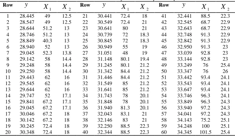
In order to investigate outlier observations through the mean-shift outlier model, the F-statistic for each observation is given in Table 4. It can be seen that 1st and 3rdobservations have larger F values than the table

Table 2. Fresh data for weekly sales of shampoos and prices

Row

y

1

X

₂ Row

y

X

₁

X

₂ Row

y

X

₁

X

₂

1 34.481 101.3 25.3 6 34.308 104.9 26.2 11 34.780 108.5 27.1 2 34.369 102 25.5 7 34.402 105.6 26.4 12 34.875 109.1 27.3 3 34.268 102.7 25.7 8 34.479 106.9 26.6 13 34.963 109.9 27.5 4 34.160 103.5 25.9 9 34.580 107 26.8 14 35.540 110.6 27.7 5 34.215 104.2 26.1 10 34.682 107.7 27 15 35.173 111.3 27.8

Table 3. Summary of descriptive statistics for shampoos and prices

Data n

y

X

₁

X

₂

Mean Standard

Deviation Mean

Standard

Deviation Mean

Standard Deviation

Historical 60 31.35 1.79 75.05 15.94 19.86 3.9

Fresh 15 34.59 0.32 106.35 3.19 26.59 0.8

Table 4. F-statistic for mean-shift outlier model

Obs. F p-value Obs. F p-value

1 6.66 0.0085 8 0.11 0.8966

2 1.72 0.2126 9 0.01 0.9901

3 4.54 0.0287 10 0.23 0.7973

4 2.99 0.0808 11 0.39 0.6837

5 0.26 0.7745 12 0.43 0.6583

6 0.01 0.9901 13 0.60 0.5615

(8)

2,n p 2

3.68

F

_{ }



at





0.05

, so these observations will be diagnosticated as outliers.

To investigate influential observations using the case deletion method, the related diagnostic measures are given in Figure 1. The cutoff points are

2

n



0.46

for DFBETAS and

2

p n

 

p

0.69

for DFFITS (see Seber [23], p.307). While the absolute values of DFBETAS and DFFITS for 8th observation are at least three times more than those for the other observations, none of these measures exceed the cutoff points and no influential observation is recognized (the above influence measures cannot be evaluated for 1st and 15th observations).

In order to identify the efficiency of our methods, a reduction shift for dependent variable, equal to 0.4 can be chosen (which is slightly more than one standard deviation of y) and exerted on 8th observation. We emphasize that this observation is more likely influential under reduction shift according to the position of 8th point in Figure 1. Table 5 shows that applying the mean-shift outlier model to the shifted dataset, the 8thobservation is recognized as an outlier, but it is observed that 7thobservation is also discerned as an outlier. According to the Remark 2, the reason is disbanding the autoregressive structure of data by shifting 8thobservation implying that these observations are outliers in accordance with the autoregressive nature of data. Again, for more investigation, a proposed

Figure 1. (a) DFBETAS for



₁, (b) DFBETAS for



₂ (c) DFFITS for fitted values after fitting Mixed Stochastic restricted Autocorrelated Ridge model to the shampoo data. The dashed lines are cutoff points.

Figure 2. (a) DFBETAS for



1, (b) DFBETAS for



2 (c) DFFITS for fitted values after fitting Mixed Stochastic Autocorrelated Ridge model to the shampoo data with a shift in 8th observation. The dashed lines are cutoff points.

Table 5. F-statistic for mean- shift outlier model after changing 8th observation

Obs. F p-value Obs. F p-value

1 1.16 0.34 8 15.84 0.00

2 0.46 0.64 9 2.5 0.12

3 0.99 0.39 10 0.14 0.87

4 0.71 0.51 11 0.22 0.81

5 0.07 0.93 12 0.24 0.79

6 0.0002 0.99 13 0.33 0.72

(9)

reduction shift equal to



ˆ



S D y

( )

is exerted on 7th observation and the result of this relief action shows that, only 8thobservation was recognized as an outlier. In other words, the shift exerted to 7th observation recovers the destroyed autocorrelated connection between the two observations.

By the reduction shift action for 8th observation, as expected, substantial changes occur in the outcome of diagnosing influential observations (see Figure 2). It can be seen that DFBETAS and DFFITS of 8thobservation exceed the cutoff points. So, in the shifted dataset, 8th observation is an influential observation.

Simulation Study

In this section the performance of the proposed methods are investigated through a simulation study. We generate data with autocorrelated error terms taking into account different values of



, sample size, degree of collinearity and shift values. Then the mean-shift outlier and the case deletion methods are conducted.

In order to produce autocollinear explanatory variables, the formula



₂



1 2

, 1

1- , 1,..., , 1,...,

ij ij i p

x   d d  i  n j  p

suggested by McDonald and Galarneau [25] is used where

d

_ijare independent standard normal

pseudo-random numbers and



is specified so that the correlation between any two explanatory variables is given by



2.

The dataset is generated based on the model

1,...,

t t t

y



x





u

t



n

with

u

_t





u

_t_₁





_t. For 40,100, 200

n , define 0.5 , 0.9,

d

_ij



N

(0, 5)

,

1 2

'

(

,

)

(0.6 , 0.4)





 







,





0.6 , 0.9

and



_t is generated from

N

(0,1)

.

Each data set is produced by a combination of model specification and generating the error terms



_t, then 40% of the sample sizes are assigned to historical data (i.e. 16, 40, 80) and 60% to fresh data (i.e. 24, 60, 120). Then the assigned data are centered and scaled by the unit normal scaling technique. The DW statistic for each set of data is calculated to assure that the autocorrelated property is still hold.

This procedure is replicated 1000 times by generating new error terms



_t, for each combination of model specification and using the assigned historical data, the estimates of



and P matrices are obtained. Then the mixed stochastic restricted ridge estimator (4) is calculated. Following Bayhan and Bayhan [6], a subset of



n 2



thand



n 2 1



thobservations of transformed historical data are used as the stochastic linear restrictions (2), so 1 ˆ

ˆ 1

W 



 

  

 

. The ridge parameter

estimate

k

ˆ

is calculated as suggested by Firinguetti [21] from assigned fresh dataset.

For each of the generated dataset the method of mean-shift outlier model for testing

H

_₂

:



_t



0

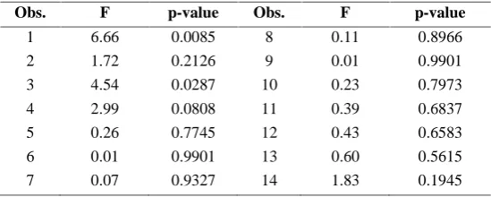
is applied and the percentage of times that the F-statistic is greater than the corresponding critical F value for

Table 6. The probability of type I error (





0.05

) and power of F test for the mean-shift outlier model with a combination of parameters n,



,



for

(

 

₁

,

₂

)



(0.6, 0.1)

and shift=3.5 and 4

n-total n





Sig level Power

Historical Fresh Shift=3.5 Shift=4

40 16 24

0.5 0.6 0.100 0.821 0.876

0.9 0.065 0.826 0.872

0.9 0.6 0.104 0.843 0.894

0.9 0.063 0.830 0.879

100 40 60

0.5 0.6 0.058 0.950 0.975

0.9 0.048 0.958 0.984

0.9 0.6 0.050 0.944 0.986

0.9 0.051 0.960 0.991

200 80 120

0.5 0.6 0.059 0.964 0.989

0.9 0.044 0.982 0.999

0.9 0.6 0.050 0.966 0.989

(10)

0.05





is calculated.

For each generated data set, the 4th observation is considered as an outlier by exerting two shift values 3.5 and 4, which are around the mean of standard deviation of generated dependent observations, to its original dependent values. The autocorrelated structure of errors is tested again by calculating the DW statistic to assure this property still hold. The power of test is calculated by the foregoing method and the results of this simulation study for different combinations of model specifications are given in Table 6.

Table 6 indicates that except for simultaneous small values of



and n, in other combinations of n,



and



the significance level remains around





0.05

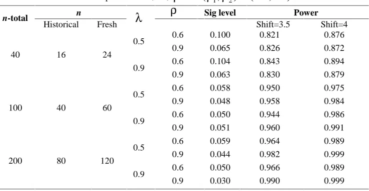
. Moreover, it shows that the power of the test is increasing continuously with increase of the shift values.

In case-deletion method, the mean of absolutes of DFBETAS, DFFITS and the proportion of replications which exceed the related cutoff points in 1000 replicates are used as judgment tools. The results of different shift values are shown in Tables 7 and 8.

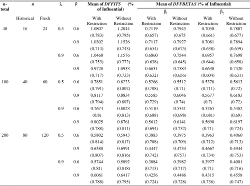
Some related results from this study are presented as

follows:

- It can be seen that the mean of

DFFIT S

and

DFBET A S and their related proportions for the mixed stochastic autocorrelated ridge regression model are smaller than the measures for autocorrelated ridge regression model. It may be due to improved accuracy of the advanced model and its reduced sensitivity to the observations which do not have a large displacement from the bulk of data.

- Increment in



does not have a significant effect on the mean of

DFFITS

and the related proportion in the small sample sizes for the both models, whereas for large sample sizes, it mainly causes a growth in the measures. These results are somehow valid for the mean

of

DFBETA S

and related proportions.

- Increment in degree of collinearity which is delegated by



has mainly a reduction effect on the mean of

DFFIT S

and the related proportion for both models. These results are somehow valid for the mean of DFBETA S and related proportions.

Table 7. Mean and proportion (%) of

DFFITS

and

DFBETAS

of 4thobservation for different values of n,



and



when Shift=3.5

n-total

n   Mean of DFFITS (%

of Influential)

Mean of DFFBETAS (% of Influential)

1

 2

Historical Fresh With

Restriction

Without Restriction

With Restriction

Without Restriction

With Restriction

Without Restriction

40 16 24 0.5 0.6 0.9429

(0.7)

1.0395 (0.73)

0.6017 (0.594)

0.6624 (0.609)

0.6681 (0.629)

0.7280 (0.646) 0.9 0.9115

(0.668)

1.0175 (0.7)

0.5902 (0.584)

0.6629 (0.613)

0.6298 (0.604)

0.6970 (0.625) 0.9 0.6 0.8940

(0.671)

0.9901 (0.689)

0.6046 (0.574)

0.6697 (0.59)

0.5981 (0.569

0.6615 (0.604) 0.9 0.9111

(0.672)

1.0267 (0.704)

0.6375 (0.6)

0.7132 (0.62)

0.6161 (0.582)

0.6917 (0.616)

100 40 60 0.5 0.6 0.6787

(0.752)

0.7114 (0.759)

0.4299 (0.634)

0.4509 (0.646)

0.4886 (0.654)

0.5123 (0.672) 0.9 0.7271

(0.767)

0.7879 (0.788)

0.5052 (0.691)

0.5471 (0.703)

0.4955 (0.678)

0.5368 (0.698) 0.9 0.6 0.6772

(0.746)

0.7079 (0.758)

0.4667 (0.659)

0.4869 (0.662)

0.4887 (0.659)

0.511 (0.676) 0.9 0.6967

(0.722)

0.7617 (0.751)

0.4845 (0.656)

0.5311 (0.679)

0.4901 (0.654)

0.5357 (0.677)

200 80 120 0.5 0.6 0.5127

(0.775)

0.5241 (0.781)

0.3380 (0.652)

0.3454 (0.658)

0.3549 (0.66)

0.3628 (0.662) 0.9 0.5344

(0.764)

0.5662 (0.782)

0.3763 (0.695)

0.3982 (0.708)

0.3717 (0.678)

0.3931 (0.694) 0.9 0.6 0.4905

(0.732)

0.5023 (0.734)

0.3412 (0.646)

0.3497 (0.655)

0.3466 (0.653)

0.3544 (0.65) 0.9 0.5313

(0.763)

0.5649 (0.774)

0.3793 (0.694)

0.4043 (0.699)

0.3830 (0.688)

(11)

- Increment in the sample size n has similar effects on the mean ofDFFITS , the mean of DFBETA S and the related proportions as follows. Almost for all of the cases it causes a significant reduction in both

DFFITS and DFBETA S , whereas it usually causes the related proportions increases, since the cutoff points are dependent on n.

- Increment in the size of shift values causes the measures and related proportions increase in all cases.

Discussion

In this article we extended the mean-shift outlier model, DFFITS and DFBETAS measures to the case of autocorrelated ridge regression model under stochastic linear restrictions. We applied our results to a real dataset with AR(1) error terms and stochastic linear restrictions. We observed that the proposed mean-shift

outlier model is efficient for detecting observations which do not conform to the nature of data which are known as outliers. Also, the derived measures are suitable for diagnosing influential observations. In addition, a simulation investigation conducted to study the performance of mean-shift outlier method showed that if shift values increase, the power of the mean-shift F test will also increase. Also, a simulation was carried out to study the behavior of DFFITS and DFBETAS for the cases of mixed stochastic autocorrelated ridge regression model and autocorrelated ridge model. This simulation study demonstrated that, in general, the influence measures in the first model are smaller than those in the second model. A reduction occurs mainly when the degree of collinearity increases, whereas increasing autocorrelation coefficient for large sample sizes causes mainly a growth in the measures and, increasing sample size almost always causes a reduction in the measures.

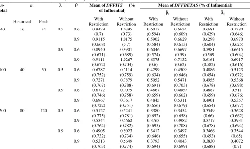
Table 8. Mean and proportion (%) of DFFITS and DFBETAS of 4thobservation for different values of n,



and



when Shift=4

n-total

n   Mean of DFFITS (%

of Influential)

Mean of DFFBETAS (% of Influential)

1

 2

Historical Fresh With

Restriction

Without Restriction

With Restriction

Without Restriction

With Restriction

Without Restriction

40 16 24 0.5 0.6 1.0807

(0.783)

1.2044 (0.795)

0.7119 (0.657)

0.7945 (0.675

0.7058 (0.661)

0.7807 (0.677) 0.9 1.0302

(0.714)

1.1526 (0.743)

0.7117 (0.654)

0.7927 (0.675)

0.7081 (0.638)

0.7894 (0.659) 0.9 0.6 1.0468

(0.753)

1.1576 (0.772)

0.6860 (0.638)

0.7544 (0.645)

0.6957 (0.644)

0.7698 (0.658) 0.9 0.9728

(0.717)

1.0933 (0.733)

0.6631 (0.632)

0.7383 (0.656)

0.6638 (0.604)

0.7420 (0.631)

100 40 60 0.5 0.6 0.7851

(0.791)

0.8223 (0.802)

0.5266 (0.708)

0.5512 (0.71)

0.5378 (0.711)

0.5613 (0.72)

0.9 0.8117 (0.794)

0.8834 (0.807)

0.5585 (0.729)

0.6046 (0.74)

0.5677 (0.7)

0.6183 (0.72) 0.9 0.6 0.7674

(0.8)

0.8023 (0.813)

0.5110 (0.688)

0.5341 (0.698)

0.5265 (0.681)

0.5482 (0.69)

0.9 0.8025 (0.788)

0.8761 (0.811)

0.5612 (0.694)

0.6141 (0.732)

0.5690 (0.71)

0.6197 (0.724)

200 80 120 0.5 0.6 0.5802

(0.814)

0.5943 (0.817)

0.3883 (0.708)

0.3975 (0.709)

0.3963 (0.712)

0.4060 (0.713) 0.9 0.6580

(0.807)

0.6991 (0.816)

0.4447 (0.742)

0.4734 (0757)

0.4667 (0.734)

0.4944 (0.753) 0.9 0.6 0.5744

(0.81)

0.5892 (0.818)

0.3884 (0.713)

0.3982 (0.717)

0.3977 (0.71)

0.4081 (0.716) 0.9 0.6061

(0.788)

0.6417 (0.795)

0.4256 (0.724)

0.4486 (0.728)

0.4315 (0.736)

(12)

Finally, in this paper we concentrated on the case deletion methods in restricted autocorrelated ridge models. This work can be extended in different directions. One direction is to study the local influence of observations in the above mentioned model. The other direction is using different biased estimators including Liu estimators and Lasso estimators.

Regarding the possible limitations, the main obstacle was that the authors had no access to the suitable real data sets from national research studies.

Acknowledgement

The authors would like to thank the editor and anonymous referees for several helpful comments and suggestions, which resulted in a significant improvement in the presentation of this paper.

References

1. Hoerl A.E. and Kennard R.W. Ridge regression: biased estimation for non-orthogonal problems. Technometrics,

12: 69–82 (1970).

2. Belsley D.A., Kuh E. and Welsch R.E. Regression

diagnostics: identifying data and sources of collinearity.

John Wiley & Sons, New York, (2004).

3. Rao C.R., Toutenburg H., Shalabh and Heumann C. Linear

models and generalizations, Least squares and alternatives. Springer, Berlin, (2008).

4. Sarkar N. A new estimator combining the ridge regression and the restricted least squares methods of estimation.

Commun. Stat.-Theor M, 21: 1987–2000 (1992).

5. Özkale M.R. A stochastic restricted ridge regression estimator. J. Multivar Anal., 100: 1706–1716 (2009). 6. Bayhan G.M. and Bayhan M. Forcasting using

autocorrelated errors and multicollinear predictor variables. Comp. ind. Eng., 34(2): 413-421 (1998). 7. Alkhamisi M.A. Ridge estimation in linear models with

autocorrelated errors. Commun. Stat.-Theor M, 39: 2630–

2644 (2010).

8. Groβ J. Restricted ridge estimation.Stat. Probabil. Lett., 65:

57-64 (2003).

9. Alheety M.I. and Golam Kibria B.M. A Generalized stochastic restricted ridge regression estimator. Commun.

Stat.-Theor M, 43: 4415–4427 (2014).

10. Chatterjee S. and Hadi A.S. Influential observations, high leverage points, and outliers in linear regression. Stat.

Science, 1(3): 379–416 (1986).

11. Roy S.S. and Guria S. Regression diagnostics in an autocorrelated model. Braz. J. Probab. Statist., 18: 103–

112 (2004).

12. Özkale M.R. and Acar T.S. Leverages and influential observations in a regression model with autocorrelated errors. Commun. Stat.-Theor M, 44: 2267–2290 (2015). 13. Acar T.S and Özkale M.R. Influence measures in ridge

regression when the error terms follow an AR(1) process.

Comput. Stat., 31(3): 879–898 (2016).

14. Ghapani F., Rasekh A.R., Akhoond M.R. and Babadi B. Detection of outliers and influential observations in linear ridge measurement error models with stochastic linear restrictions. J. Sci. I. R. Iran, 26(4): 355 - 366 (2015). 15. Wang J. Statistical diagnosis of linear regression model

with the random constraints and Bayes method. Nanjing

University of Science and Technology, Nanjing, (2007). 16. Wen H.W. and Wing K.F. The mean-shift outlier model in

general weighted regression and its applications. Comp.

Stat. data an., 33(4): 429-441 (1999).

17. Pan J. and Xiong H. Outliers and influential observations in a ridge mean shift regression, System science and

Mathematical science, 9(1): 12-26 (1995).

18. Ghapani F., Rasekh A.R. and Babadi B. Mean shift and influence measures in linear measurement error models with stochastic linear restrictions. Comm. Stat-Simulat.C.,

46(6): 4499-4512 (2017).

19. Theil H. and Goldberger A.S. On pure and mixed statistical estimation in economics. Int. Econ. Rev., 2 : 65-78 (1961).

20 Troskie C.G., Chalton D.O., Stewart T.J. and Jacobs M. Detection of outliers and influential observations in regression analysis using stochastic prior information,

Commun. Stat.-Theor M, 23(12): 3453–3476 (1994). 21. Firinguetti L. A simulation study of ridge regression

estimators with autocorrelated errors. Commun. Stat.

Simulat., 18(2): 673-701 (1989).

22. Judge G.C., Hill R.C., Griffiths W.E., Lütkepohl H. and Lee T.C. Introduction to the Theory and Practice of

Econometrics. John Wiley & Sons, New York, (1988).

23. Seber G.A.F. and Lee A. Linear Regression Analysis. John Wiley & Sons, New Jersey, (2003).

24. Montgomery D.C., Peck E.A., and Vining G.G. Linear

Regression Analysis,5th Ed., John Wiley & Sons, New Jersey, (2012).

26. McDonald G.C. and Galarneau D.I. A monte carlo evaluation of some ridge type estimators. J. Am. Stat.