Welfare Effects of
Short-Time Compensation
*
Helge Braun
aBj¨
orn Br¨
ugemann
b, c*January 2017
Abstract
We study welfare effects of public short-time compensation (STC) in a model in which firms
respond to idiosyncratic profitability shocks by adjusting employment and hours per worker.
Intro-ducing STC substantially improves welfare by mitigating distortions caused by public unemployment
insurance (UI), but only if firms have access to private insurance. Otherwise firms respond to low
profitability by combining layoffs with long hours for remaining workers, rather than by taking up
STC. Optimal STC is substantially less generous than UI even when firms have access to private
insurance, and equally generous STC is worse than not offering STC at all.
Keywords: Short-Time Compensation, Unemployment Insurance, Welfare JEL Classification: J65
*We are grateful to Klaudia Michalek for her participation in early stages of the project. We would like to thank Pierre Cahuc, Rob Euwals, Moritz Kuhn, and numerous seminar and conference participants for helpful comments and discussions.
aRuhr Graduate School in Economics.
bVU Amsterdam, Tinbergen Institute, CESifo, and IZA.
cCorresponding author at: VU Amsterdam, Department of Economics, De Boelelaan 1105, 1081 HV Amsterdam, Netherlands.
1
Introduction
Virtually all developed countries have public unemployment insurance (UI) systems. In addition, many
countries run public short-time compensation (STC) schemes, which pay benefits to workers that have
not lost their job but are working reduced hours. In contrast to UI, STC has not been a universal
component of social insurance systems in developed countries. Before the 2008-2009 crisis, STC schemes
existed in 18 out of 33 OECD countries. Such schemes increased in popularity during the crisis, with
many countries expanding existing schemes and others introducing new schemes on a temporary basis.1
This increase in the popularity of STC has also revived academic interest in this policy instrument.
Recent research has primarily focussed on employment effects of STC during the crisis.2 What has
received little attention, both in recent and earlier work, are effects of STC on social welfare. This
contrasts with UI, which has been studied extensively from a welfare perspective. In this paper we study
welfare effects of STC in a setting in which UI is socially optimal, consistent with the observation that
UI is a universal feature of social insurance systems in developed countries. We ask if introducing STC
can improve welfare in a situation in which the instrument of UI is already used optimally.
We study this question in a static model of implicit contracts, building on existing theoretical work
on STC. Workers are risk averse and ex ante heterogeneous in that they are either attached to a firm
or unattached. Both attached and unattached workers can be unemployed ex post. We follow existing
work in not separating the role of workers and employers: workers attached to a firm are both suppliers
of its labor input as well as its owners. Firms are subject to idiosyncratic profitability shocks, and can
adjust through a combination of layoffs and work sharing in the sense of adjusting hours per worker.
Profitability shocks are interpreted as temporary, and layoffs are interpreted as temporary layoffs that
do not break attachment to the firm. The government has two policy instruments, UI and STC. UI is a
payment to each unemployed worker, where a worker is considered unemployed if working zero hours.3
Thus workers are unemployed either because they are unattached or on temporary layoff. UI is the only
source of income for unattached workers. STC is a payment for each hour by which working time is
reduced below some threshold of normal hours. We allow for the possibility that eligibility for STC may
require a minimum reduction in hours per worker, a common feature of existing STC schemes.4 The
1Arpaia et al.(2010) andHijzen and Venn(2011) survey STC schemes.
2See for exampleArpaia et al.(2010),Hijzen and Venn(2011),Boeri and Bruecker(2011),Cahuc and Carcillo(2011), Hijzen and Martin(2013), andBalleer et al.(2016).
3Unemployment here means eligibility for benefits rather than search activity. Unattached workers are eligible. For consistency with the typical UI system, their status should be interpreted as including having worked in the recent past.
government balances the budget through a linear tax on total hours.
When studying public insurance, it is important to take into account agents’ access to private
insur-ance (PI). The premise of implicit contract models is that firms are an important source of PI, due to
firms’ superior access to financial markets relative to workers. Firms are heterogeneous in the extent of
this access, however, and we are interested in how the extent of access to PI affects the response of firms
to the availability of STC, and in turn the welfare effects of STC. For simplicity, we restrict attention to
two polar scenarios: either firms have access to perfect PI, or they have no access to PI.5
Welfare effects of UI in this setting are well understood. It has a positive effect on utilitarian welfare
via redistribution towards unattached workers. If firms lack access to perfect PI, UI also provides
insurance to attached workers. The cost of UI is a distortion of labor inputs, as firms do not internalize
the impact of layoffs on the government budget (Feldstein,1976).
Starting from a situation in which the level of UI is chosen to maximize social welfare, the introduction
of STC can affect welfare through two channels. First, since private labor input decisions are distorted
by UI, STC affects welfare through its impact on these decisions. This is the only welfare effect of STC
when firms have access to perfect PI. If firms lack such access, STC also has a direct insurance effect,
since it reallocates resources across firms with different realizations of profitability.
Our analysis proceeds in two main steps. First, we analyze firms’ decisions for given values of
the policy instruments. In particular, we characterize how firms adjust labor inputs in response to
profitability shocks, conditional on the decision to take up STC. This is well known for the case of
perfect PI: when profitability is sufficiently low for layoffs to be optimal, a further drop in profitability
causes lower employment, while hours per worker remain constant. For the case of no PI and for our
specification of preferences, which is a standard specification in macroeconomics, we establish a new
comparative statics property: the availability of UI induces firms to respond to a drop in profitability
by increasing hours per worker. This occurs because lower profitability raises the marginal utility of
consumption relative to the marginal disutility of working longer hours for workers with positive hours.6
hours reductions. They range from 4% to 40%, with an average around 20%.
5In implicit contract models that separate the roles of workers and employers, the extent of a firm’s access to PI is usually captured indirectly via the risk aversion of the employer, with risk neutrality at one end of the spectrum. In contrast, we model access to PI directly.
This property turns out to be key in shaping the welfare effects of STC when firms lack access to PI.
In the second step, we study welfare-maximizing choices of UI and STC. We rely on computational
experiments, calibrating the model by targeting features of the US labor market. We obtain two main
results. First, introducing STC substantially improves welfare, but only if firms have access to PI. If
firms have such access, STC can mitigate excessive layoffs caused by UI. This mechanism fails if firms
lack access to PI, due to the comparative statics property discussed above. In the absence of STC,
unprofitable firms would choose layoffs combined withhighhours per worker, and this makes the take-up
of STC unappealing. Instead, STC is taken up by firms with intermediate profitability, and for most
of these firms STC merely distorts hours. This pattern of take-up also implies that STC has a direct
negative insurance effect, but quantitatively this is relatively unimportant. Overall, adopting the same
level that is optimal in the case of PI leads to a moderate welfare loss. Thus our model suggests that
to the extent that the government can observe firms’ access to PI, it is desirable to have different levels
of STC for different groups of firms. Our second main result is that optimal STC is substantially less
generous than UI even when firms have access to PI. In our model there is no reason to expect that
equal generosity is optimal, since the optimal levels of STC and UI are governed by different trade-offs:
as discussed above, optimal UI is governed by the trade-off between the benefits of redistribution and
insurance and the cost of inducing excessive layoffs, while optimal STC balances the benefit of reducing
these excessive layoffs against the cost of distorting hours in firms that would abstain from layoffs even
in the absence of STC. According to our computational experiments, STC should be about one third
as generous as UI. Furthermore, equally generous STC is worse than not offering STC at all. This is
important, given that equal generosity of STC and UI is a common feature of existing schemes.7
We contribute both to the literature using implicit contract models to study STC, and the broader
literature using such models to study the response of layoffs and hours per worker to shocks. Our analysis
of STC builds heavily onBurdett and Wright(1989, henceforth BW) and Wright and Hotchkiss(1988,
henceforth WH). BW use an implicit contract model to study effects of UI and STC on layoffs, hours per
worker, and wages. A key feature of their model is that laissez faire is socially optimal. Their analysis
is focussed on the distortions induced by UI and STC. They find that while UI distorts the level of
employment, STC distorts hours per worker. WH extend the analysis of BW in several directions, two
of which are important for our purposes. While BW consider a model in which workers and employers
are distinct agents, WH also consider a simplified model which abstracts from this heterogeneity. We
adopt this simplification. Second, WH use this simplified model to analyze social welfare. As in BW,
having neither UI nor STC is socially optimal. Alternatively, UI and STC can be neutralized through
full experience rating. If there is no UI in their model, then it is also optimal to have no STC. Neither
BW nor WH address the question whether a positive level of STC would be optimal given that the level
of UI is positive. Addressing this question is important, given that UI is universal across developed
economies. Our main contribution to this literature is to fill this gap. We generate a reason for the
existence of UI through the presence of unattached workers.8 In turn, the existence of UI gives rise to a nontrivial trade-off for STC, since STC can mitigate distortions induced by UI.
Since the work of BW and WH on STC, there has been tremendous progress in the development
of dynamic models of the labor market. Nonetheless, static implicit contract models remain a natural
starting point for studying the welfare effects of STC because they combine the following three
fea-tures: (i) specificity of employment relationships, captured by the attachment of workers to firms, (ii)
multi-worker firms, adjusting at both the extensive and the intensive margin, (iii) private insurance
arrangements among the agents attached to a firm, in a setting with incomplete markets. While there
are dynamic models capturing these features individually, tractable models capturing them jointly have
not yet been developed. Of course, a static model does not allow us to evaluate some potential effects
of STC, such as the concern that STC reduces the reallocation of workers to more productive firms.9
Tilly and Niedermayer(2016) analyze employment and welfare effects of STC with a different focus,
developing a dynamic model with heterogeneous workers that successfully captures several micro-level
facts concerning STC take-up in Germany. This focus on dynamics and heterogeneity comes at the
cost of assuming single-worker firms. Thus they do not consider a central feature in BW’s and our
analysis: multi-worker firms deciding how to spread reductions in total hours across layoffs and work
sharing. A second key difference concerns private insurance. They argue that for Germany it is realistic
to restrict employment contracts to an hourly wage, which furthermore cannot respond to temporary
shocks in ongoing jobs. While employers are risk neutral, this limits their ability to insure workers. This
inefficiency may explain why they find an optimal STC replacement rate close to 100% in their model.
8When firms lack access to perfect PI, an additional source of welfare gains from UI and potentially STC in our model is insurance provision against idiosyncratic profitability shocks. In contrast, in both BW and WH shocks are aggregate and thus undiversifiable, whether through public or private insurance.
Our contribution to the broader implicit contracts literature is the comparative statics property
discussed above, which applies when firms lack access to PI and public UI is available: if profitability
is sufficiently low for layoffs to be optimal, then a firm responds to a further reduction in profitability
by reducing employment andincreasing hours per worker. Rosen (1985) andFitzRoy and Hart(1985)
study the corresponding comparative statics for the case of perfect PI, and show that hours are constant
across profitability levels for which layoffs are optimal. The analysis closest to ours is Miyazaki and
Neary (1985), who study the comparative statics of employment and hours for a firm without access
to PI. They find that an increase in profitability can reduce both employment and hours per worker if
firms have to cover fixed costs that are independent of employment, or if income effects are sufficiently
strong. Our finding differs in that a change in profitability induces an opposite response of employment
and hours, and that this pattern is induced by the presence of UI, which acts like a fixed cost per worker.
Blanchard and Tirole (2008) use a mechanism design approach to study optimal UI in a model
with constant hours per worker. The key friction is that profitability is private information of the
employer. They find that constrained efficiency generally requires that public insurance is exclusive, that
is, supplementary UI provided by employers must be restricted. In contrast, we restrict the government
to the instruments of UI and STC described above, and supplementary UI (and STC) by firms is
unrestricted. It would be interesting to generalize Blanchard and Tirole’s mechanism design approach to
a setting with variable hours. Blanchard and Tirole also study optimal UI when firms’ access to financial
markets is limited, specifically by having shallow pockets. This resembles our case of imperfect PI, but
the implications in their setting are quite different.10
The remainder of the paper is organized as follows. We introduce the model in Section2. In Section
3we characterize the allocation for a given system of UI and STC. Section4contains the computational
experiments. Section5considers an alternative specification of technology, and Section6concludes.
2
Model
There is a continuum of firms, each with a massN of workers attached and jointly owned and operated
by these workers. We normalizeN = 1. A fractionυ of the total population of workers is unattached.
Technology. Each firm has the production function xf(nh) where n denotes the mass of workers
working strictly positive hours, hdenotes the number of hours worked by each of these workers, and
xparametrizes the profitability of the firm. The function f : [0,+∞)→[0,+∞) is twice continuously
differentiable withf′>0 andf′′<0 on (0,+∞), and satisfies the Inada conditions liml→0f′(l) = +∞
and liml→∞f′(l) = 0. Profitabilityxis subject to stochastic shocks that can be of technological or other
origin, with densityp(x) and support (0,+∞).
Hours per worker and employment enter multiplicatively, thus hours of different workers are perfect
substitutes. This specification is used by WH, and dubbed thestandard caseby BW. BW also study a
specification with imperfect substitutability. We maintain the standard case for most of our analysis. In
Section5 we consider the case in which hours of different workers are perfect complements.
Preferences. The utility function of a worker isE[u(c, h)], wherecdenotes consumption andhdenotes
hours worked. The functionutakes the form proposed byKing et al. (1988, KPR):
(1) u(c, h) = [cv(h)]
1−σ−1
1−σ
with σ > 1. The function v : [0, hmax) →(0,1] satisfies v(0) = 1. Here hmax ∈ (0,+∞] is a physical
upper limit on hours. The function v incorporates a fixed utility loss from working strictly positive
hours: limh→0v(h) =v0withv0∈(0,1). The functionvis twice continuously differentiable and satisfies
v′<0 on (0, hmax). We assume that −v
′
v is strictly increasing on (0, hmax) to ensure that consumption
is a normal good. LetV(h)≡ −v(h)1−σ2σv′(h). We assume V′(h)>0 to ensure that u(c, h) is strictly
concave, and we impose the Inada condition limh→hmaxV(h) = +∞.
Our specification is more general than BW in that we allow for a fixed utility loss from working
strictly positive hours. It is less general than BW in that the KPR functional form restricts the relative
strength of income and substitution effects. The KPR functional form is standard in macroeconomic
models, since it is necessary for balanced growth. We see this paper as a step towards incorporating
STC in a dynamic macroeconomic model, making this functional form a natural choice.
Private Insurance. We consider two polar cases, parametrized byχ ∈ {0,1}. If χ = 0, firms have
access to perfect PI. Ifχ= 1, firms have no access to PI.
Policy Instruments. UI takes the form of a payment gU I >0 to workers with zero hours worked.
STC takes the form of a paymentgST C ≥0 to employed workers for every hour that hours worked fall
short of some normal level ¯h. We impose the restriction ¯hgST C ≤gU I, so the maximal amount of STC,
obtained by working marginally positive hours, cannot exceed the level of UI. The normal level ¯h is
schemes require a minimum hours reduction (MHR). To capture this feature, firms are eligible for STC if
hours are belowgM HR¯h, wheregM HR≤1. The government balances the budget through a proportional
taxτ >0 on total hoursnh. Thus a firm with employmentnand hourshreceives the net subsidy
(2) (1−n)gU I+nI
[
h≤gM HR¯h
]
·(¯h−h)·gST C−τ nh
where I denotes the indicator function. Unattached workers receive the UI benefit gU I. Notice that
this system of UI and STC is uniform: it does not differentially treat workers based on the profitability
of their firm, nor does it distinguish between attached and unattached workers. We do not model the
reasons why the government does not use differential benefits.
This policy specification is based on BW and WH, and generalizes theirs in three ways. First, they
simplify the analysis by assuming that the normal level of hours ¯h coincides with the physical upper
limit hmax. This implies that in their models firms always receive STC, allowing them to ignore the
decision of whether to take up STC. We allow ¯hand hmax to differ. To pin down ¯hwe require that in
equilibrium it equals the average level of hours across states of the world. Second, BW restrict attention
to two regimes: an American regime withgST C = 0, and a European regime in which UI and STC are
equally generous, that is, ¯hgST C =gU I. We allow any value of gST C between 0 and equal generosity.
While many countries have equal replacement rates for UI and STC, in some countries STC is effectively
less generous. For example, German firms pay social security contributions for hours not worked due
to take-up of STC. In our computational experiments it turns out that equal generosity is not optimal.
Third, in their specification firms receive STC whenever hours are below the normal level ¯h, which, as
discussed above, coincides with the physical upper limithmaxin their model. We introduce the parameter
gM HR to investigate whether a minimum hours reduction is a desirable feature of STC schemes.
BW assume that the government balances the budget through a lump sum tax. In their setup without
a relevant eligibility threshold, this is isomorphic to our specification with a proportional tax on total
hours.11 This is no longer true in our setup with an eligibility threshold. Given this, we prefer the proportional tax, since it mimics more closely the observed financing of UI through payroll taxes.12
Our specification does not include so-called experience rating, which requires that a firm reimburses
the government for part of the UI and STC benefits received by its workers. Exactly as in the models
11 Without the eligibility threshold, net subsidy schedule (2) reduces to (1−n)g
of BW and WH, experience rating is redundant in our model: in Appendix Bwe show that a system
with experience rating is equivalent to a system without experience rating and lower benefits. Thus we
can omit experience rating without loss of generality. When mapping the model to the data, gU I and
gST C should be interpreted as subsidies net of any experience rating. Furthermore, the restriction that
UI and STC are uniform should be understood as a restriction on net subsidies.13
Firm Optimization Problem. Let T(x)∈ {0,1} indicate the decision of the firm to take up STC
in statex. Let ι(x) denote the net transfer received from PI in state x. The firm choosescw(x),cb(x),
n(x),h(x),ι(x), andT(x) for allx∈(0,+∞) to maximize
(3)
∫ ∞
0
{n(x)u(cw(x), h(x)) + (1−n(x))u(cb(x),0)}p(x)dx
subject to
n(x)cw(x) + (1−n(x))cb(x) =xf(n(x)h(x)) +ι(x)−τ n(x)h(x)
(4)
+(1−n(x))gU I+n(x)
(¯
h−h(x))T(x)gST C,
n(x)≤1,
(5)
T(x)·(h(x)−gM HR¯h
) ≤0,
(6)
χι(x) = 0 (7)
for allx∈(0,+∞) and
(8)
∫ ∞
0
ι(x)p(x)dx= 0.
Constraint (8) requires that PI is actuarially fair. Ifχ= 1, then (7) enforces that the firm has no access
to PI by requiringι(x) = 0 in every state.
Government Optimization Problem. We restrict the government to choose the vector of policy
instrumentsg ={gU I, gST C, gM HR,¯h, τ
}
from a set G. By varying G, we can restrict the set of policy
instruments available to the government. In our computational experiments, we consider a sequence
of expanding sets G, to examine the added value of introducing the policy instrument STC with and
without a minimum hours requirement. The objective function of the government is utilitarian welfare,
giving weightυto unattached workers.14 LetU(g) denote the maximized value of the firm optimization
problem as a function of the policy vector, and letcw(x, g),cb(x, g),n(x, g),h(x, g),ι(x, g), andT(x, g)
denote corresponding maximizers. Given these functions, the government choosesg∈ G to maximize
(9) (1−υ)U(g) +υu(gU I,0)
subject to the government budget constraint
(10)
∫ ∞
0
{
(1−n(x, g))gU I+n(x, g)
(¯
h−h(x, g))T(x, g)gST C−τ n(x, g)h(x, g)
}
p(x)dx= 0
and the constraint that normal hours coincide with average hours per worker
(11) ¯h=
∫∞
0 ∫n(x, g)h(x, g)p(x)dx
∞
0 n(x, g)p(x)dx
.
First-Best Optimization Problem. A useful reference point for the allocations chosen by the
gov-ernment is the first-best allocation. It is obtained by choosingcw(x),cb(x),n(x),h(x), and unattached
workers’ consumptioncν to maximize utilitarian welfare
(1−ν) ∫ ∞
0
{n(x)u(cw(x), h(x)) + (1−n(x))u(cb(x),0)}p(x)dx+νu(cν,0)
subject to constraint (5) and the resource constraint
(1−ν) ∫ ∞
0
{n(x)cw(x) + (1−n(x))cb(x)−xf(n(x)h(x))}p(x)dx+νcν= 0.
If firms have access to perfect PI, the only reason why the government cannot achieve the first best
is that attached workers on layoff are not excluded from UI. If firms lack access to PI, then a second
reason is that its policy instruments do not permit conditioning transfers directly on profitabilityx.
3
Optimal Firm Behavior
In this section we analyze the firm optimization problem, proceeding in three steps. In Section3.1 we
derive first-order conditions and obtain comparative statics properties of optimal hours. In Section3.2
we analyze how optimal labor inputs vary with profitability conditional on the decision to take up STC.
That is, we fix the take-up decision, and study optimal labor input profiles separately for the cases of
take-up and no take-up of STC. In Section3.3we combine these results to discuss the take-up decision.
3.1
First-Order Conditions
Letλ(x)p(x),ν(x)p(x),ζ(x)p(x),ρ(x)p(x), andµdenote the multipliers associated with constraints (4),
(5), (6), (7), and (8). The first-order conditions forcw(x),cb(x),n(x),h(x), andι(x) are
uc(cw(x), h(x)) =λ(x),
(12)
uc(cb(x),0) =λ(x),
(13)
u(cb(x),0)−u(cw(x), h(x)) =λ(x)
[
xf′(n(x)h(x))h(x)−cw(x) +cb(x)
(14)
−gU I+
(¯
h−h(x))T(x)gST C−τ h(x)
]
−ν(x),
−n(x)uh(cw(x), h(x)) =λ(x)
[
xf′(n(x)h(x))n(x)−n(x)T(x)gST C−τ n(x)
]
−T(x)ζ(x),
(15)
λ(x) =µ+ρ(x)χ.
(16)
Conditions (12)–(13) imply that consumption levels of employed and unemployed workers arecw(x) =
c∗w(λ(x), h(x)) andcb(x) =c∗b(λ(x)), respectively, withc∗w(λ, h)≡λ− 1/σ
v(h)(1−σ)/σ andc∗b(λ)≡λ−1/σ. Next, we analyze the first-order conditions that determine the optimal level of hours per worker. We
first consider the case in which the employment constraint (5) is slack, and then turn to the case in which
it binds. In both cases we focus on the case in which constraint (6) is slack, since its impact on optimal
hours is straightforward. If the constraints (5) and (6) are slack, that is, ifν(x) = 0 andζ(x) = 0, then
combining first-order conditions (14) and (15) yields
(17) u(cb(x),0)−u(cw(x), h(x)) +uh(cw(x), h(x))h(x) =λ(x)
[
cb(x)−cw(x)−gU I+ ¯h·T(x)gST C
]
.
This is the first-order condition for a variation that reduces employment while increasing hours per worker
hto keep total hours nhconstant. The left-hand side gives the utility gain from this variation. Each
worker now has a larger chance of being on layoff, which yields the utility gainu(cb(x),0)−u(cw(x), h(x)).
To keep total hours constant, the additional layoff must be compensated by redistributingh(x) hours
across the remaining workers, which yields a utility loss of −uh(cw(x), h(x))h(x). The right-hand side
gives the impact of this variation on the budget constraint. The additional worker on layoff is switched
T(x)gST C in STC for the worker on layoff, and an additional h(x)·T(x)gST C due to higher hours for
remaining workers, for a total of ¯h·T(x)gST C.
Substituting the functionsc∗w andc∗b, we obtain a condition linking hours and the multiplierλwhich
does not directly involve profitabilityx:
(18) u(c∗b(λ),0)−u(c∗w(λ, h), h) +uh(cw∗(λ, h), h)h+λ
[
c∗w(λ, h)−c∗b(λ) +gU I−hT¯ ·gST C
] = 0.
The following proposition establishes that this equation has a unique solution for hours, and characterizes
the comparative statics of hours with respect toλandT. All proofs are collected in AppendixA.
Proposition 1 Equation (18)has a unique solution forhgiven anyλ >0andT ∈ {0,1}. IfgST C >0,
then this solution is strictly decreasing inT. If gU I−¯hT ·gST C >0, then it is strictly increasing in λ.
If gU I−¯hT ·gST C = 0, then it is independent of λ.
Hours are decreasing in T if gST C > 0, since gST C subsidizes low hours. The relationship between
the multiplier λ and hours is less obvious. In the absence of a net payment from the government
(gU I−¯hT ·gST C = 0), hours are determined by the trade-off between the fixed disutility of working
positive hours and the increasing marginal disutility of working long hours. Higher fixed costs favor
longer hours, while convex disutility favors spreading hours across many workers. With KPR utility,
the optimal level of hours determined by this trade-off is not affected by the multiplier λ. UI benefits
introduce an additional fixed cost of working positive hours, incurred in terms of the consumption good.
A higher multiplier λ indicates that consumption is more valuable. This shifts the trade-off in favor
of higher hours. Thus UI distorts the composition of labor inputs in the direction of higher hours and
lower employment. If taken up, STC counteracts this distortion and eliminates it entirely if UI and
STC are equally generous, that is, if ¯hgST C =gU I. The property that hours are strictly increasing in
λ if gU I−¯hT ·gST C > 0 and independent of λ ifgU I−¯hT ·gST C = 0 also holds for other common
specifications of utility. In particular, it also holds when utility is additively separable in consumption
and hours. With GHH preferences, hours are independent ofλeven ifgU I−¯hT·gST C >0.15
The key implication of equation (18) is that hours are affected by profitability xonly through the
multiplierλ(x), which is the marginal utility of consumption. With perfect PI,λ(x) does not vary with
profitability, hence hours are constant. As we discuss below, without PIλ(x) is decreasing inx, hence
hours are declining inx. Thus firms experiencing an uninsured decline in profitability and engaging in
layoffs have relatively high hours for those workers that remain at work.
Next, consider the case in which the employment constraint is binding. Substitutingn(x) = 1 along
with the functionc∗winto first-order condition (15) yields
−uh(c∗w(λ, h), h) =λ[xf′(h)−τ−T·gST C].
Substituting the functional forms ofuh andc∗w yields
(19) V(h) =λσ1[xf′(h)−τ−T·gST C].
The following proposition establishes that this equation has a unique solution for hours, and characterizes
the comparative statics of hours with respect tox,λ, andT.
Proposition 2 Equation (19)has a unique solution forhgiven anyx >0andT∈ {0,1}. This solution
is strictly increasing in xandλ, and converges to hmax asxconverges to infinity. IfgST C >0, then it is strictly decreasing in T.
UI does not directly affect the choice of hours when the firm does not engage in layoffs.
3.2
Labor Input Profiles Conditional on STC Take-Up
In this section we analyze how optimal labor inputs vary with profitability conditional on STC take-up,
separately for the cases of perfect PI and no PI. Let h0(x) and n0(x) denote the levels of hours and
employment that would be optimal if STC is not taken up. Here the superscript indicates thatT = 0.
Analogously, leth1(x) andn1(x) denote the corresponding levels if STC is taken up, that is, ifT = 1.
3.2.1 Perfect Private Insurance
Proposition 3 If χ = 0, then the functionsh0(x), n0(x), h1(x), and n1(x) are continuous and have the following properties.
1. There exists a thresholdx0
N ∈(0,+∞)such thath0(x)is constant on
( 0, x0
N
)
and strictly increasing
on (x0 N,+∞
)
, whilen0(x)is strictly increasing on(0, x0 N
)
and equal to one on(x0 N,+∞
)
.
2. There exist thresholdsx1N ∈(0,+∞)andx1M HR∈[xN1,+∞]such thath1(x)is constant on(0, x1N), strictly increasing on(x1N, x1M HR), and constant atgM HR¯hon
(
x1M HR,+∞), whilen1(x)is strictly increasing on (0, x1
N
)
and equal to one on (x1 N,+∞
)
.
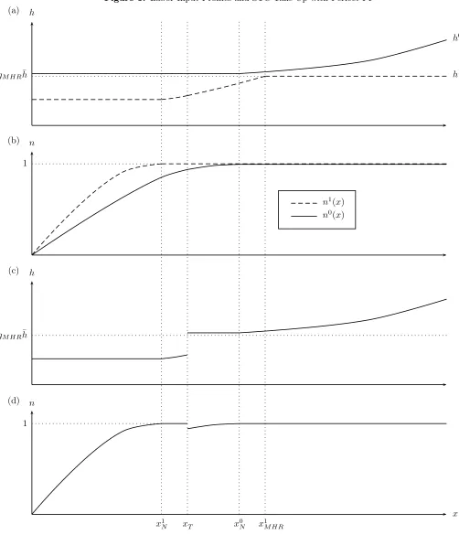
Figure 1: Labor Input Profiles and STC Take-Up with Perfect PI
x n
(d)
h
(c)
n
(b)
h
(a)
x0 N
x1
N x
0
T x
1 M HR
h0(x)
h1(x)
gM HR¯h
1
n1(x)
n0(x)
gM HR¯h
This proposition is illustrated in Panels (a) and (b) of Figure1. Part 1 characterizesh0(x) and n0(x).
There are two profitability regions across which the qualitative behavior of labor inputs differs, divided
by a thresholdx0
N at which the employment constraint becomes binding. Below this threshold the firm
engages in layoffs, and hours per workers are constant. The latter follows directly from Proposition
1, which states that hours do not vary with profitability xconditional on the multiplier λ(x). Perfect
PI implies that λ(x) is independent ofx, hence hours are constant. Employment is strictly increasing
over this region. Abovex0N the behavior of hours is governed by Proposition 2. Hours are now strictly increasing in profitability as it is no longer possible to take advantage of higher profitability by raising
employment. This characterization of labor input profiles in the case of perfect PI is well-known, and
can be found inRosen(1985),FitzRoy and Hart(1985), andBurdett and Wright(1989), among others.
Part 2 of the proposition describes h1(x) and n1(x). Again there is a threshold x1
N at which the
employment constraint becomes binding, and the qualitative behavior of labor inputs above and below
this threshold is very similar to the case of no take-up. The only difference stems from the MHR
constraint. Abovex1
N, hours are strictly increasing in profitability until the MHR constraint is binding.
It is also possible that the MHR constraint is already binding belowx1
N, in which case hours do not vary
with profitability over the entire profitability range (0,+∞).
Part 3 shows that hours under take-up are always below hours under no take-up. In essence, this
follows directly from the comparative statics for hours with respect to take-up established in Propositions
1and2.16 Part 3 is silent on the relative position of the employment schedules n0(x) andn1(x).
First-order condition (14) shows that take-up provides an employment subsidy of (¯h−h)gST C per worker,
which by itself increases employment. The effect of take-up on employment is ambiguous, however, as
the reduction in hours induced by take-up reduces the marginal product from employing an additional
worker.17 In particular, it is ambiguous whether n0(x) or n1(x) attains one first, that is, the relative
position of the thresholds x0
N and x1N is also ambiguous. In our computational experiments the case
n1(x)> n0(x) always prevails, which impliesx1N < x0N. This case is illustrated in Panel (b) of Figure1.
3.2.2 No Private Insurance
Proposition 4 If χ = 1, then the functionsh0(x), n0(x), h1(x), and n1(x) are continuous and have the following properties.
1. There existsx0N ∈[0,+∞] such thath0(x)is strictly decreasing on(0, x0N)and strictly increasing 16Proposition1implies this result for profitability below min[x0
N, x1N], and Proposition2does so for the region above max[x0
N, x 1
N]. The only extra work in the proof of Part 3 of Proposition3is to establish this result betweenx 0 N andx
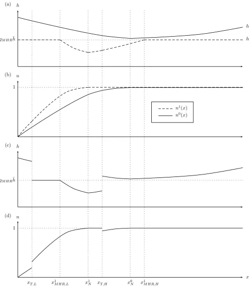
Figure 2: Labor Input Profiles and STC Take-Up without PI
x n
(d)
h
(c)
n
(b)
h
(a)
x0 N
x1
N x
1 M HR,H
x0
T ,H
x1 M HR,L
x0
T ,L
h0(x)
h1(x)
gM HR¯h
1
n1(x)
n0(x)
gM HR¯h
on (x0 N,+∞
)
, whilen0(x)is strictly increasing on(0, x0 N
)
and equal to one on(x0 N,+∞
)
.
2. There exist x1
N ∈ [0,+∞], x1M HR,L ∈ [0, x1N], and x1M HR,H ∈ [x1N,+∞] such that h1(x) is constant at gM HRh¯ on
( 0, x1
M HR,L
)
, weakly decreasing on (x1
M HR,L, x1N
)
, strictly increasing on
(
x1
N, x1M HR,H
)
, and constant atgM HR¯hon(x1M HR,H,+∞). It is strictly decreasing on
(
x1 M HR,L,
x1 N
)
if gU I−¯hgST C >0. n1(x)is strictly increasing on(0, x1N)and equals one on
(
x1 N,+∞
)
.
3. IfgST C >0, thenh1(x)< h0(x)for all x∈(0,+∞).
This proposition is illustrated in Panels (a) and (b) of Figure 2. Employment schedules behave
quali-tatively as in the case of perfect PI. In contrast, the behavior of hours is different. Consider first the
case of no take-up. The profileh0(x) is strictlydecreasingbelow the thresholdx0
N. This is explained by
Proposition1, according to which hours are strictly increasing in the multiplierλifgU I−¯hT·gST C>0,
which holds if STC is not taken up. In the absence of PI the multiplierλ, which coincides with marginal
utility of consumption, is strictly decreasing in x.18 This carries over to hours. As explained in the
discussion of Proposition1, λ affects optimal hours through its interaction withgU I, which acts like a
fixed cost of employment in terms of the consumption good. Consumption is scarce after an uninsured
decline in profitability. The optimal response of the firm is to send workers to collect UI benefits, which
is one way of obtaining consumption, and to implement longer hours for workers that remain on the
job.19 This comparative statics result is new to the implicit contracts literature.20 In Section4we show that it has important implications for the welfare effects of STC.
Hours are strictly increasing inxabove the full-employment thresholdx0
N. Qualitatively, this is as in
the case of perfect PI, but the economic forces are somewhat different. With perfect PI, the increase in
hours is purely driven by a substitution effect, thus our assumption of KPR preferences is not important
for this result. In contrast, here the marginal utility of consumption is decreasing in profitability, hence
the response of hours depends on the relative strength of income and substitution effects. With KPR
preferences these effects would cancel exactly in the absence of policy, that is, ifτ = 0. A positive taxτ
makes the income effect relatively weaker, hence the substitution effect dominates.
The hours profile conditional on take-up of STC h1(x) is qualitatively similar to h0(x). As in the case of perfect PI, its shape only differs due to the MHR constraint. However, the hours profile would be
V-shaped in the absence of the MHR constraint. This implies that in general there are two profitability
18This is established in the course of the proof of Proposition4.
19Notice that we have assumed that all fixed costs of employment accrue in terms of utility, so that UI is the only fixed cost in terms of consumption. If other fixed costs also accrue in terms of consumption, then this strengthens the result.
intervals over which the MHR constraint binds. First, below a threshold x1
M HR,L, which lies in the
profitability range with a slack employment constraint. Second, above a thresholdx1
M HR,H, which lies
in the profitability range over which the employment constraint binds.
Part 3 establishes that, as in the case of perfect PI, take-up reduces hours.
3.3
STC Take-Up
Having analyzed labor input profiles conditional on take-up, we now discuss optimal take-up. Consider
first the case of perfect PI. The next proposition gives sufficient conditions such that take-up is monotone
in profitability, occurring at low levels of profitability.
Proposition 5 Suppose thatχ= 0andgST C >0. Iff(nh) = (nh)αwithα∈(0,1) andx1N < x0N, then there existsxT ∈[0,+∞] such that optimal take-up isT∗(x) = 1on (0, xT]andT∗(x) = 0 on(xT,∞).
The first condition is that the technology is Cobb-Douglas, which we employ in our computational
experiments. The second condition is that the employment constraint starts to bind at a lower level
of profitability in the case of take-up, that is, x1 N < x
0
N. As discussed in the context of Proposition 3,
x1 N < x
0
N prevails in all our computational experiments, although the reverse is a theoretical possibility.
The monotonicity of optimal take-up in Proposition5is driven by the complementarity between total
hours nT(x)hT(x) and profitability. Take-up is associated with a reduction in hours. Everything else
equal, this leads to lower total hours. This can be countered by an increase in employment, but only if
the employment constraint is slack. Once profitability is sufficiently high, firms taking up STC run into
the employment constraint. This makes take-up more costly, the more so the higher is profitability.
The take-up thresholdxT can lie anywhere in [0,+∞]. Panels (c) and (d) of Figure 1 illustrate the
optimal labor input profiles for the case in whichxT lies between the two employment thresholds x1N
andx0N. They are generated from Panels (a) and (b) by selecting the take-up schedulesh1(x) andn1(x) to the left of xT, and the no take-up schedules h0(x) and n0(x) to the right of xT. As x increases,
hours are first flat while employment increases. Hours start to increase as the employment constraint
becomes binding under take-up atx1
N. Next, hours jump up and employment jumps down at the take-up
thresholdxT. After that, hours are once again flat while employment increases until the employment
constraint becomes binding under no take-up atx0
N. Beyond this point, hours are once again increasing.
Next, consider the case of no PI. Here we have no theoretical results for take-up, as the analysis
is substantially complicated by income effects. As with perfect PI, one force is that take-up is more
costly if higher hours would be optimal conditional on no take-up. With perfect PI, this gives rise to the
up. Since the latter are monotone inx, so is take-up. For illustration, suppose that this force remains
dominant in shaping take-up. The key difference to perfect PI is that hours are not monotone inx, but
V-shaped. Thus one would expect no take-up to occur in two separate regions of profitability, both at
very low and very high levels ofx. Panels (c) and (d) of Figure2illustrate such a case with two take-up
thresholds, denoted xT ,L and xT ,H. The lower take-up threshold xT ,L is located in the profitability
region over which hours conditional on take-up are strictly declining inx, both forT= 1 andT = 0. In
the case illustrated here, the second take-up threshold is located betweenx1N andx0N, when hours are still strictly decreasing inxconditional on no take-up, but are already strictly increasing in profitability
conditional on take-up due to a binding employment constraint. The labor input schedules in Panels
(c) and (d) are generated from Panels (a) and (b) by selecting the no-take schedulesh0(x) andn0(x) to
the left and to the right of xT ,L andxT ,H, respectively, and the take-up schedulesh1(x) andn1(x) in
between. Hours jump down and employment jumps up atxT ,L, the reverse happens atxT ,H.
4
Computational Experiments
In this section we carry out computational experiments to examine whether introducing STC can improve
on a system restricted to UI in our model. We obtain two main results. First, whether STC can improve
on UI depends critically on firms’ access to PI. STC substantially improves welfare if firms have access to
perfect PI, but yields only a negligible improvement when firms lack access to PI. Under perfect PI, STC
improves welfare by reducing excessive layoffs induced by UI. This mechanism is greatly diminished if
firms lack access to PI, because the most distressed firms prefer long hours over taking up STC. Second,
the optimal generosity of STC is substantially below that of UI even with perfect PI, and introducing
STC with equal generosity results in a large welfare loss in comparison to having no STC at all.
4.1
Calibration
We calibrate the model to match features of the US labor market. The functional form off is
f(nh) = (nh)α.
We setα= 2
3, implicitly assuming that capital cannot be adjusted in response to profitability shocks.
For the utility function given in equation (1) above, we specify
v(h) = exp (
−ηh
1+ψ
1 +ψ+ log (v0)I[h >0]
)
where η and ψ are strictly positive. The parameterη only affects the level of hours, so we can use it
to normalize employment-weighted average hours to one. We set the coefficient of relative risk aversion
to σ = 2, within the “plausible” range 1–5 indicated by micro estimates, see Heathcote et al. (2009).
The parameter ψ governs the Frisch elasticity of labor supply. Based on the recent survey of the
microeconomic evidence inHall(2009), we target a Frisch elasticity of 0.7.21 We setυ= 0.045, so that
4.5% of workers are not attached to a firm. Together with the level of temporary layoffs targeted below,
this matches the average unemployment rate in the US of about 6%.
The densityp(x) is log-normal. We normalize the mean of log(x) to zero and set its standard deviation
to σx = 0.1, a reasonable order of magnitude for firm-specific shocks for a time horizon between six
months and one year, see for exampleComin and Philippon(2006) andDavis et al.(2007).
We calibrate an economy that has UI but no STC. Thus two parameters remain to be calibrated:
v0, which governs the fixed utility loss from working strictly positive hours, and the UI benefitgU I. We
jointly calibrated them to match two targets. First, we target that 1.5% of all workers experience a
temporary layoff. Thus 25% of all the unemployed are attached. We base this target on the empirical
prevalence of temporary layoffs. In the US Current Population Survey, on average 14% of the stock
of unemployed workers is classified as on temporary layoff.22, 23 Fujita and Moscarini (2016) find that temporary layoffs are relatively more important for flows, accounting for one third of the flow from
employment to unemployment. Our target strikes a balance between the importance of temporary
layoffs for flows and stocks, as our static model cannot match them separately. Second, we target a UI
replacement rate of 25%, where we define the replacement rate in the model asgU Idivided by the average
consumption of workers. Recall that experience rating is neutral in our model andgU I corresponds to
the UI subsidy net of experience rating. Topel(1983) reports that on average the net subsidy is 31% of
earnings. In our model workers jointly own and operate firms, hence implicitly their average consumption
reflects income from both wages and profits. This leads us to adopt the somewhat lower target of 25%.
These targets pin downgU I and v0 as follows. BothgU I andv0 act as a fixed cost of working positive
hours. The fraction of workers on temporary layoff is increasing in fixed costs, so the corresponding
target pins downv0 for givengU I. We then varygU I to match the targeted replacement rate.
21The Frisch elasticity is(ψ+σ−1 σ
(
ηh1+ψ))−1. At average hours, this reduces to(ψ+σ−1 σ η
)−1
.
22The average is taken over the years 1967-2012.
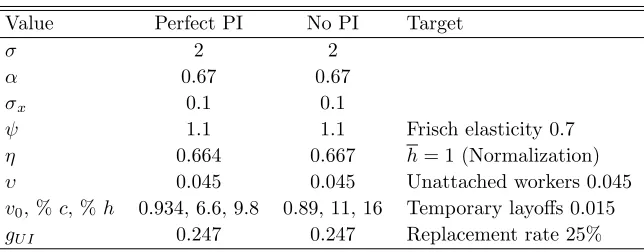
Table 1: Calibration: Perfect PI and No PI
Value Perfect PI No PI Target
σ 2 2
α 0.67 0.67
σx 0.1 0.1
ψ 1.1 1.1 Frisch elasticity 0.7
η 0.664 0.667 h= 1 (Normalization)
υ 0.045 0.045 Unattached workers 0.045
v0, %c, %h 0.934, 6.6, 9.8 0.89, 11, 16 Temporary layoffs 0.015
gU I 0.247 0.247 Replacement rate 25%
The calibration for both cases, perfect PI and no PI, is summarized in Table1. The policy parameter
gU I is pinned down quite directly by the replacement rate target. Only the utility fixed costv0 differs
substantially between the two calibrations. With perfect PI it equals 0.934, which corresponds to 6.63%
in terms of consumption and 9.76% in terms of hours.24 Its value is higher in the case of no PI,
corresponding to 11% in terms of consumption. Lack of insurance makes firms more reluctant to carry
out layoffs, thus the fixed cost must be higher to match the targeted level of temporary layoffs. In an
appendix toBraun and Br¨ugemann(2017), we show that the main results obtained in the remainder of
this section are insensitive to changes in parameters and targets over a wide range of values.
We carry out the following sequence of policy experiments, summarized in Table2. Each experiment
is defined by restrictions on the set of policy instrumentsG in the government optimization problem of
Section2. First, we restrict this set to UI and determine the welfare-maximizing level ofgU I. We denote
this asgU I∗ , and also useg∗U Ito label this experiment. We usegU I∗ rather than the calibrated level ofgU I
as the starting point for experiments that introduce STC. Otherwise welfare gains from STC could merely
reflect a suboptimal level ofgU I, rather than a genuine added value ofgST C as a policy instrument. The
next three experiments introduce STC without a minimum hours requirement, hencegM HR= 1. In the
first, we determine the optimal level ofgST C holding constantgU I atgU I∗ . By construction, introducing
gST C in this way does not affect the level of consumption of unattached workers. Therefore, to the extent
that STC does improve the allocation, it can only do so by mitigating the distortion of labor inputs
induced byU I. We refer to the corresponding level of STC and also the entire experiment asg∗ST C|g∗U I
to indicate thatgST C∗ is optimal conditional on fixing the level of UI atgU I∗ . In the second experiment,
we introduce a level of gST C that is as generous as g∗U I. This level satisfies gST C¯h = gU I∗ , and the
corresponding experiment is labeled gmax
ST C|g∗U I. In the next step, we determine the welfare-maximizing
24The cost associated withv
Table 2: Policy Experiments
Policy Experiment Restrictions on the Set of Policy InstrumentsG Remarks
gU I∗ gST C = 0,gM HR= 1
gST C∗ |gU I∗ gU I=gU I∗ , gM HR= 1
gmax
ST C|gU I∗ gU I=gU I∗ , gST Ch=g∗U I,gM HR= 1 Perfect PI only
(gU I, gST C)∗ gM HR= 1
(gST C, gM HR)∗|g∗U I gU I=gU I∗
(gU I, gST C, gM HR)∗ None
gST C|g∗U I
gU I=gU I∗ , gST Ch/gU I takes same value as in
No PI only experimentg∗ST C|g∗U I under perfect PI,gM HR= 1
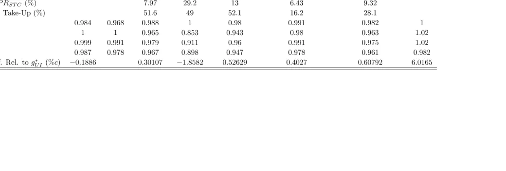
Table 3: Policy Experiments: Perfect PI
Calibr. g∗U I g∗ST C|g∗U I gmax
ST C|g∗U I (gU I, gST C)∗ (gST C, gM HR)∗|g∗U I (gU I, gST C, gM HR)∗ FB
gU I 0.247 0.262 0.262 0.262 0.284 0.262 0.28
gST C 0.08 0.308 0.13 0.0643 0.0933
gM HR 1 1 1 0.81 0.82
τ 0.0158 0.0214 0.0196 0.0501 0.0278 0.017 0.0237
REP RU I (%) 25 26.7 27.1 29.2 29.9 26.8 29.1
REP RST C (%) 7.97 29.2 13 6.43 9.32
STC Take-Up (%) 51.6 49 52.1 16.2 28.1
¯
n 0.984 0.968 0.988 1 0.98 0.991 0.982 1
¯
h 1 1 0.965 0.853 0.943 0.98 0.963 1.02
¯
y 0.999 0.991 0.979 0.911 0.96 0.991 0.975 1.02
¯
c 0.987 0.978 0.967 0.898 0.947 0.978 0.961 0.982
Welf. Rel. to g∗U I (%c) −0.1886 0.30107 −1.8582 0.52629 0.4027 0.60792 6.0165
combination of gST C and gU I denoting this experiment as (gU I, gST C)∗. The next two experiments
introduce an MHR by allowing gM HR do differ from one. First, in the experiment (gST C, gM HR)∗|g∗U I
we once again fix the level of U I at g∗U I while jointly choosinggST C and gM HR optimally. Finally, in
the experiment (gU I, gST C, gM HR)∗ we choose all three policy instruments optimally.
4.2
Perfect Private Insurance
Results for the case of perfect PI are in Table3. The calibration and the first best (FB) are shown as
points of reference. For each experiment, the first six rows show the values of the policy instruments
gU I, gST C and gM HR, and the tax τ, along with the replacement rates implied by gU I and gST C,
labeled REP RU I and REP RST C, respectively.25 The next row reports the STC take-up rate, that
is, the average fraction of attached workers receiving ST C in percent. The next four rows show the
average of employment and average (employment weighted) hours for attached workers, denoted ¯nand
¯
h, respectively, along with average output ¯y and consumption c across attached workers. The final row
shows, for each allocation, the welfare gain vis-`a-vis the experimentg∗U I. Here and in the remainder of
the paper, welfare gains are expressed in percentage consumption-equivalent terms. Figure3 compares
labor input profiles for the three experimentsg∗U I,gST C∗ |g∗U I, and (gU I, gST C)∗and the first best. These
correspond to the theoretical labor input profiles of Figure 1, showing hours and employment as a
function of profitabilityx.26 Thick gray segments indicate the region of STC take-up.
ExperimentgU I∗ shows that optimal UI is somewhat above the calibrated level.27 The corresponding
level of ¯nis 0.968, compared to 0.984 in the calibration. Thus the number of workers on layoff doubles.
Hence layoffs respond quite strongly to gU I, a point we return to below. Employment is below one at
sufficiently low levels of profitability and increasing. Hours are constant over the profitability range with
positive layoffs and increasing otherwise, as established in Part 1 of Proposition3. In contrast, first-best
employment is one irrespective of profitability, and first-best hours are increasing throughout.
Experiment g∗ST C|g∗U I shows that introducing STC is optimal when UI is fixed atgU I∗ , and it
estab-lishes half of our first main result: under perfect PI, STC can substantially improve welfare, here by
0.3%. The optimal level of gST C is modest: the implied replacement rate for STC is 7.97%, compared
25REP R
U I is defined as the ratio betweengU I and average consumption, expressed in percentage terms. Analogously,
REP RST C is defined as the ratio between the maximal STC benefitgST C¯hand average consumption. Thus the two replacement rates coincide ifgST C¯h=gU I.
26The x-axis is scaled to the distribution of profitability shocks.
Figure 3: Hours and Employment, Perfect PI
0.79 0.88 0.93 1.00 1.06 1.13 1.26
0.8 0.9 1 1.1 1.2 h
x
0.79 0.88 0.93 1.00 1.06 1.13 1.26
0.5 0.6 0.7 0.8 0.9 1 n
x g∗
U I
g∗ STC|gU I∗ (gU I, gSTC)∗ FB
to 27.1% for UI. Nevertheless, this level of STC is quite effective, reducing layoffs by more than half.
As discussed in Section3.2.1, an increase in employment is not implied by our theoretical analysis, but
occurs in all of our computational experiments. Hours per worker drop substantially, so that output is
lower than in experiment gU I∗ , despite higher employment. Lower spending on UI outweighs spending
on STC, and government outlays as a percentage of output are reduced from 2.19% under experiment
gU I∗ to 2%. The labor input profiles for this experiment conform to Propositions 3and 5. The take-up
thresholdxT lies above the threshold xN0 at which the employment constraint becomes binding under
no take-up.28 Thus some firms taking up STC would have retained all workers even in the absence of
STC. For these firms STC distorts hours without the benefit of reducing layoffs. Employment is then
continuous at the take-up threshold, while hours jump up. Throughout the take-up region, hours are
strictly lower than in experimentgU I∗ and employment is uniformly higher.
In experimentgmax
ST C|g∗U I, STC eliminates layoffs completely, but induces a very large decline in hours.
Overall, this leads to a large welfare loss of 1.85% vis-`a-vis experimentgU I∗ . Together with the preceding
experiment, this establishes our second main result: Optimal STC is substantially less generous than
UI, and introducing STC with equal generosity results in a large welfare loss in comparison to having no
STC at all. In our model there is no natural reason for UI and STC to be equally generous. The optimal
levels of UI and STC are determined by different trade-offs. Optimal UI balances the benefit of making
Figure 4: Welfare Gains and Average Labor Inputs as Functions ofgST C, Perfect PI
−1.5 −1 −0.5 0
❣ ♠❛① ❙❚❈
✁✂✄ ❲❡❧❢☎r ❡●☎✐ ♥❘❡❧✳ t♦✆
↕ ❯■
❇❡♥❝❤✝☎r❦ ❋r✐ s❝❤❂✵✳✷
0.85 0.9 0.95 1
❣ ♠❛① ❙ ❚❈
✁✂✄ ✞
0.85 0.9 0.95 1
❣ ♠❛① ❙❚❈
✁✂✄ ✟
transfers to unattached workers against the cost of distorting the layoff decision of firms. Optimal STC
balances mitigation of this distortion against the cost of distorting hours in firms that would abstain from
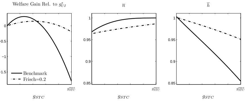
layoffs even in the absence of STC. Figure4illustrates this result. The left panel plots the welfare gain
as a function ofgST C, withgU I fixed atgU I∗ andgST C varying up togST Cmax. The middle and right panel
show how average employment and hours vary withgST C. STC is quite effective in eliminating layoffs,
in that employment already approaches the maximum level of one at intermediate levels ofgST C. In
contrast, average hours are falling linearly ingST C. When pushed beyond intermediate levels, few layoffs
are left to eliminate, while the negative effect on average hours is undiminished. Thus the optimal STC is
substantially belowgST Cmax, andgST Cmax yields a large welfare loss. For further intuition, the dashed-dotted
lines in Figure4repeat the experiment with the model recalibrated to match a lower Frisch elasticity of
0.2. In this case firms are less willing to reduce hours in response to more generous STC. Thus layoffs
are eliminated less quickly as gST C increases. The optimal generosity of STC relative to UI is higher,
yet the associated welfare gains are substantially lower.29
Experiment (gU I, gST C)∗ shows that the optimal combination of UI and STC involves substantially
more generous UI than under experiment g∗U I: the benefit level gU I increases by more than 8% (from
0.262 to 0.284), which corresponds to an increase in the replacement rate from 27.1% to 29.9%. STC
mitigates the distortions associated with UI, which in turn makes it optimal to offer more generous
UI. Thereby the availability of STC improves insurance indirectly. As in experiment gST C∗ |gU I∗ , STC
is substantially less generous than UI. The welfare gain of moving from gU I∗ to (gU I, gST C)∗ is 0.53%.
Figure 5: Hours and Employment, Perfect PI: Minimum Hours Reduction
0.79 0.88 0.93 1.00 1.06 1.13 1.26
0.8 0.9 1 1.1 1.2
h
x
0.79 0.88 0.93 1.00 1.06 1.13 1.26
0.5 0.6 0.7 0.8 0.9 1
n
x
g∗ U I
(gSTC, gM HR)∗|gU I∗ (gU I, gSTC, gM HR)∗ FB
About half of this gain can be obtained by moving tog∗ST C|g∗U I, indicating that adjusting the level of UI
is equally important to reap the full benefit of having STC as an additional instrument. Qualitatively
the pattern of labor inputs across profitability in Figure3 is very similar to the experiment g∗ST C