Evaluating Default Policy: The Business Cycle Matters
Supplementary Appendices
Grey Gordon
Indiana University
November 8, 2014
A
Data and Calibration [For Online Publication]
This appendix describes the data and provides additional calibration details.
A.1
Data
GDP and its components are taken from the National Income and Product Accounts (NIPA). Consumer durables are separated from consumption and added to investment. All values are converted to real values using the GDP deflator. The GDP deflator is also used to convert the nominal interest rates to real ones. For labor supply, I follow Ohanian and Raffo(2011) and take annual hours worked from the Conference Board’s Total Economy Database (TED).1
The number of households is taken from the Census Bureau’s historical tables.2
The model was constructed to capture the salient features of Chapter 7 bankruptcy in the U.S. The filing rate is thus measured as the ratio of Chapter 7 filings to the number of households. Filings data that go back to 1960 are only available on a fiscal year basis ending in June until 1990.3 To recover the annual figure ending in December for year y prior to
1990, I use the average of yand y+ 1. To test how well this works, I compare this method’s values with the known values for the period 1990-2004. This produces an R2 of .985.
Three measures of debt are used in the paper because because of data availability issues. First, I use net worth from the Survey of Consumer Finances. This is the closest measure of a−x in the model. Second, I use the Federal Reserve Board of Governors’ measures of
1Available athttp://www.conference-board.org/data/economydatabase/#files. 2Available at
http://www.census.gov/population/www/socdemo/hh-fam.html#ht(Table HH-1).
3Available at
revolving consumer credit (as well as their charge-off rates on credit cards and interest rate on two-year personal loans).4 Last, I use the unsecured debt measure inBermant and Flynn
(1999). AsBermant and Flynn(1999) only look at filers, this should be a good approximation for −a+xsince these households typically have no assets.
Call the three debt measures SCF, FRB, and BF respectively. In Table 1 of the main paper, the following debt measures are used: The “Debt-Output Ratio” is measured using SCF; the “Discharged Debt-Output Ratio” is measured using FRB charge-off rates times the FRB debt; and the “Debt-Income of Filers” is measured using BF. In Table 2 of the main paper, “Debt” is measured using FRB. Likewise, “Discharged Debt” is measured using the FRB charge-off rate times the FRB debt. Lastly, in Figure 2 of the main paper, the “Debt-Output Ratio” is measured using FRB.
Figure 1 shows the annual percent of Chapter 7 filings per household from the period 1960 to 2012. The number of households filing drastically increased starting in 1984, leveled off in the late 1990s, experienced a spike in 2005, a sharp decrease in 2006 and 2007, and a subsequent recovery.5 Unfortunately, the sample period drastically affects not only the
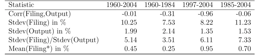
level of bankruptcies but also their cyclicality and volatility. Because of this, Table1reports statistics for the sample periods 1960-1984, 1985-2004, 1997-2004, and 1960-2004. In addition to 1984 and 2005 being breakpoints visually, these were years of substantial bankruptcy reform.6 Bankruptcy filings are between 3.5 and 7.3 times more volatile than output and are acyclical to countercyclical with a correlation between -.01 and -.96 depending on the sample period. Figure 2 plots log filings per household and log real GDP using the HP filter with parameter 100 for the sample 1960-2004. Visually, bankruptcy filings are much more volatile than output and appear to be countercyclical, but not strongly.
A.2
Calibration
There are several calibration details omitted in the main text. This section fills out those details. Table 2lists the profiles of all variables.
One omitted detail is how the sample in Karahan and Ozkan(2011) of ages 24 to 60 was
4Available at http://www.federalreserve.gov/releases/g19/HIST/default.htm and http://www.
federalreserve.gov/releases/chargeoff/chgallsa.htm. The interest rates on two-year personal loans are slightly lower than the rates on credit cards, but the time series goes back to 1972 rather than just 1994.
5Several possible explanations for the drastic rise in filings have recently been evaluated by Livshits,
MacGee, and Tertilt(2010). The spike in 2005 and subsequent sharp decrease is presumably due to antici-pation of BAPCPA clearing out potential defaulters.
6There were essentially two rounds of substantial bankruptcy legislation. The first round began with the
1960 1965 1970 1975 1980 1985 1990 1995 2000 2005 2010 0.4
0.6 0.8 1 1.2 1.4
Year
% of Hhs Filing
Percent of Households Filing
Figure 1: Chapter 7 Filings Per Household (1960-2012)
1960 1965 1970 1975 1980 1985 1990 1995 2000 2005 −0.25
−0.2 −0.15 −0.1 −0.05 0 0.05 0.1 0.15 0.2
Year
Deviation from Trend
Deviations from Trend
Pct of Filings Real GDP
Statistic 1960-2004 1960-1984 1997-2004 1985-2004
Corr(Filing,Output) -0.01 -0.31 -0.96 -0.06
Stdev(Filing) in % 10.25 7.53 8.22 11.23
Stdev(Output) in % 1.99 2.14 1.35 1.53
Stdev(Filing)/Stdev(Output) 5.14 3.51 6.11 7.33
Mean(Filing*) in % 0.45 0.25 0.95 0.70
*In levels.
Table 1: Cyclical Properties of Chapter 7 Filings per Household
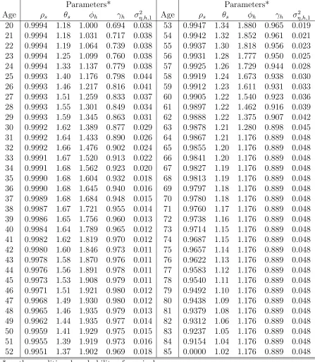
dealt with. To obtain the shock persistences for younger and older households, I assume the cubic profile is correct. To obtain the standard deviations, I assume the profile is correct for older households, but use a different approach for younger households. Specifically, I assume the standard deviation is constant for younger households and choose it so that the unconditional standard deviation at age 24 is the same as what Karahan and Ozkan(2011) find.
Another detail is how the earnings profile was constructed from the estimates ofHubbard, Skinner, and Zeldes(1994).Hubbard et al.(1994) estimate separate deterministic profiles for household heads with less than 12 years of education (NHS), 12-15 years (HS), and 16+ years (COL) of education. I average the profiles of these three types for the year 1986 assuming 13% of the population is NHS, 48% is HS, and 39% is COL. This breakdown of educational attainment is from the 2010 Current Population Survey for ages 30-34.7
Lastly, the consumption equivalence profile was constructed assuming θs =f(Ns) where
Ns is the average number of household members (the profile of which was provided to me by
Alexander Bick and Sekyu Choi) andf is the mean equivalence scale inFern´andez-Villaverde and Krueger (2007) linearly-interpolated to be continuous. This leads to a consumption equivalence profile very similar to the one in Livshits, MacGee, and Tertilt (2007).
B
Computation [For Online Publication]
This section describes the computation.
B.1
Grids
The steady state model is computed using a collection of standard techniques. The effi-ciency process is discretized using the method of Tauchen (1986). The persistent shock is
7Available athttp://www.census.gov/hhes/socdemo/education/data/cps/2010/tables.html(Table
Parameters* Parameters*
Age ρs θs φh γh σ2η,h,1 Age ρs θs φh γh ση,h,2 1
20 0.9994 1.18 1.000 0.694 0.038 53 0.9947 1.34 1.880 0.965 0.019 21 0.9994 1.18 1.031 0.717 0.038 54 0.9942 1.32 1.852 0.961 0.021 22 0.9994 1.19 1.064 0.739 0.038 55 0.9937 1.30 1.818 0.956 0.023 23 0.9994 1.25 1.099 0.760 0.038 56 0.9931 1.28 1.777 0.950 0.025 24 0.9994 1.33 1.137 0.779 0.038 57 0.9925 1.26 1.729 0.944 0.028 25 0.9993 1.40 1.176 0.798 0.044 58 0.9919 1.24 1.673 0.938 0.030 26 0.9993 1.46 1.217 0.816 0.041 59 0.9912 1.23 1.611 0.931 0.033 27 0.9993 1.51 1.259 0.833 0.037 60 0.9905 1.22 1.540 0.923 0.036 28 0.9993 1.55 1.301 0.849 0.034 61 0.9897 1.22 1.462 0.916 0.039 29 0.9993 1.59 1.345 0.863 0.031 62 0.9888 1.22 1.375 0.907 0.042 30 0.9992 1.62 1.389 0.877 0.029 63 0.9878 1.21 1.280 0.898 0.045 31 0.9992 1.64 1.433 0.890 0.026 64 0.9867 1.21 1.176 0.889 0.048 32 0.9992 1.66 1.476 0.902 0.024 65 0.9855 1.20 1.176 0.889 0.048 33 0.9991 1.67 1.520 0.913 0.022 66 0.9841 1.20 1.176 0.889 0.048 34 0.9991 1.68 1.562 0.923 0.020 67 0.9827 1.19 1.176 0.889 0.048 35 0.9990 1.68 1.604 0.932 0.018 68 0.9813 1.19 1.176 0.889 0.048 36 0.9990 1.68 1.645 0.940 0.016 69 0.9797 1.18 1.176 0.889 0.048 37 0.9989 1.68 1.684 0.948 0.015 70 0.9780 1.18 1.176 0.889 0.048 38 0.9987 1.67 1.721 0.955 0.014 71 0.9760 1.17 1.176 0.889 0.048 39 0.9986 1.65 1.756 0.960 0.013 72 0.9738 1.16 1.176 0.889 0.048 40 0.9984 1.64 1.789 0.965 0.012 73 0.9714 1.15 1.176 0.889 0.048 41 0.9982 1.62 1.819 0.970 0.012 74 0.9687 1.15 1.176 0.889 0.048 42 0.9980 1.60 1.846 0.973 0.011 75 0.9657 1.14 1.176 0.889 0.048 43 0.9978 1.58 1.870 0.976 0.011 76 0.9622 1.13 1.176 0.889 0.048 44 0.9976 1.56 1.891 0.978 0.011 77 0.9583 1.12 1.176 0.889 0.048 45 0.9973 1.53 1.908 0.979 0.011 78 0.9540 1.11 1.176 0.889 0.048 46 0.9971 1.51 1.921 0.980 0.012 79 0.9492 1.10 1.176 0.889 0.048 47 0.9968 1.49 1.930 0.980 0.012 80 0.9438 1.09 1.176 0.889 0.048 48 0.9965 1.46 1.935 0.979 0.013 81 0.9379 1.08 1.176 0.889 0.048 49 0.9962 1.44 1.935 0.977 0.014 82 0.9312 1.06 1.176 0.889 0.048 50 0.9959 1.41 1.929 0.975 0.015 83 0.9237 1.05 1.176 0.889 0.048 51 0.9955 1.39 1.919 0.973 0.016 84 0.9154 1.04 1.176 0.889 0.048 52 0.9951 1.37 1.902 0.969 0.018 85 0.0000 1.02 1.176 0.889 0.048 *ρs: the conditional probability of survival.
θs: adult-equivalent household size.
φh: deterministic earnings profile.
γh: income shock persistence.
σ2
η,h,1: persistent shock variance.
discretized with 15 points with a coverage of ±6.25 “average unconditional standard devi-ations,” ¯ση,1/
p
1−ρ¯2 (which is roughly ±5 average unconditional standard deviations in
recessions). The bar denotes the numerical average across ages. The transitory shock is dis-cretized with 5 points and a coverage of ±5 standard deviations. The right-tail process was discretized with 10 log-spaced points. The mass on each point was also computed using Tauchen (1986) (e.g., the mass on the low point is the cdf evaluated at the midpoint of the lowest two points). The asset grid (which is really the knots of a linear interpolant) is com-prised of 150 points with 60 strictly negative. These are unevenly spaced and concentrated close to zero. The household problem is solved using backward induction with linear splines (interpolants) representing continuation utilities and expenditure schedules. A grid search is first employed to avoid local minima, followed by a one-dimensional version of the simplex method.
B.2
Business Cycle Computation
The model with aggregate risk is computed using the method of Krusell and Smith (1998). The “moments” used are the capital-labor ratio and a parameter controlling the equity premium.8 The equity premium W is defined on the domain [0,1] and controls ¯q
g and ¯qb as
follows:
¯
qg(S) =
R(G) + W 1−W
F(b|z)
F(g|z)R(B) −1
and (1)
¯
qb(S) =
(1−W)
W
F(g|z)
F(b|z)R(G) +R(B) −1
(2)
whereR(S) = 1+r(S)−δ. The probabilities ensure the equilibrium value ofW is always close to, but slightly above,.5. The household problem is solved with backward induction. Linear interpolation is used to interpolate between aggregate moments (as well as in the household problem). To optimize, a grid search is used followed by a simplex algorithm (either one-dimensional or two-one-dimensional depending on the portfolio restrictions). For results to be comparable between the steady state and business cycle versions, the same number and placement of grid points are used in both models (in both the asset and efficiency direction).
8The use of the capital-labor ratio rather than capital and labor separately significantly reduces the
The laws of motion take the following form:
"
K0/N0 W0
# =
"
Γ11,zz0 Γ12,zz0 0
Γ21,zz0 Γ22,zz0 0
#
1
K/N W
(3)
Here the subscript zz0 means the coefficients are z and z0-dependent. Note thatW doesnot
influence the one-step ahead forecast. This allows the equity premium to vary holding fixed all other prices. The resulting laws of motion are very accurate for both the experiments in the main paper and the robustness tests.
Because the computational burden is heavy, especially in terms of memory usage, the number of points used for the aggregate moments is kept to a minimum: 5 in the K/N
direction linearly-spaced within ±15% of the steady-state value and 3 in the W direction placed at .50, .51, and .52. Because the natural borrowing limit and welfare depend on the worst possible scenario that can occur, and on how quickly it can be reached, the bounds and the number of grid points used can influence the results. The bounds I’ve chosen I believe are reasonable, especially given U.S. history where the capital-output ratio declined by some 20% in the Great Depression and hours worked per household has seen declines of 4% since 1960 (relative to trend).9
The model is simulated non-stochastically as in Young(2010) for 5000 periods, and the first 250 periods are discarded. At each point in the simulation, the bond market must be cleared. Because the equity premium is included in the aggregate state space, this involves linearly interpolating the asset policies to find an equilibrium W.
B.3
Computing the Transition
For computing transitions between steady states, the following algorithm is used. Let a superscript of old denote a variable associated with the original steady state and new with the new one. Let a superscript of t denote the time period.
1. Fix T, the length of the transition period.
2. Take K1 = Kold and guess on {Kt}T
t=2, a level of the capital stock for each period in
the transition.
3. Compute {q¯t, rt, wt}T
t=1 associated with the capital stock sequence.
9Author’s calculations. Hours worked per household are calculated as discussed in Appendix A. The
4. Using backward induction with VT :=Vnew, compute the value function, policy
func-tions, and price schedules for each time period. To compute Vt and a0t, one needs qt,
which is known since it depends only on dt+1 and factor prices.
5. Using forward induction, computeµt+1as a function ofµtanda0tfor each 1≤t ≤T−1.
6. Compute the implied capital stock for each t and call it ˜Kt.
7. If max2≤t≤T|Kt−K˜t|< K, go to 8. Otherwise, go to 2 with an updated guess on the
capital stock of θKKt+ (1−θK) ˜Kt for 2≤t ≤T.
8. If |K˜T −Knew|< δ
K, STOP. Otherwise, increase T and go to 1.
A transition length of T = 50 was sufficient when using δK = .001 and K = .0001. The
differences in the capital-output ratio of BAPCPA and FS are fairly small, soθK =.8 worked
without trouble.
B.4
Business Cycle Welfare Calculations
Welfare in the business cycle is computed as follows. In theKrusell and Smith(1998) method, one replaces the aggregate state variables with “moments”mand the aggregate law of motion maps moments and shocks into moments tomorrow. Linear interpolation in the moments, which performs a convex combination of adjacent values on a grid, effectively induces a prob-ability distribution over the moments tomorrow, F(m0|m, z, z0) withP
m0F(m0|m, z, z0) = 1
and F(m0|m, z, z0)≥0.10 Hence, there is an implied Markov chain F(m0, z0|m, z). The com-putational equivalent of the GX ergodic distribution in Section 4.1 of the paper is F(m, z),
the invariant distribution of the implied Markov chain.
An interesting alternative to using this unconditional F(m, z) distribution is to consider
P
sFˆ(s|z)
R
eVF S(0, e, s,0;S) ˆf(e|s, z)de
P
sFˆ(s|z)
R
eVN F S(0, e, s,0;S) ˆf(e|s, z)de
−1, (4)
which is a function ofS. One can compute the mean and standard deviation of this measure over the business cycle. If this is done, the average is close to the unconditional measure in the paper. Specifically, the average gain of moving from FS to NFS is -.125% (the unconditional measure is -.128%). The standard deviation is .110%.11
10This is only the case for interpolation. Extrapolation would result inF(m0|m, z, z0)<0.
11In fact, NFS looks better in recessions. The principle reason is simply that households want to borrow
C
Robustness [For Online Publication]
This section conducts many robustness checks. I have tried to include the most impor-tant ones, but the source code can be used for additional checks. Although there are many bankruptcy regimes in the paper, only FS and NFS are considered as they are the most different from one another and the cost of computing these checks is quite large.
C.1
An Alternative Debt Calibration
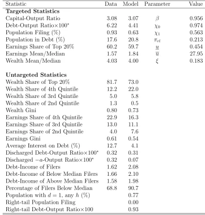
The benchmark calibration used debt statistics from Chatterjee, Corbae, Nakajima, and R´ıos-Rull (2007), which are based on net worth measures from the Survey of Consumer Fi-nances (SCF). When one uses debt measures based on revolving consumer credit, asLivshits et al. (2007) do, the debt statistics are much larger. As a robustness check, I recalibrated the model to match a debt-output ratio of 6.22 (the average revolving consumer credit to GDP ratio from 1995 to 2004, authors’ calculations) and a population in debt of 17.6 (the population with zero or negative net worth in 2001 according to Wolff, 2010) with all other targets the same. The results are presented in Table 3. The fit is not as good as in the base-line calibration. Even with the flexible default cost structure χ(e) = χ0−χ1e−1, the model
struggles to match both debt and default rates.
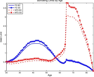
This alternative calibration has, quite naturally, a massive impact on average borrowing limits as can be seen in Figure 3. Now the average borrowing limit is typically higher in FS than in NFS with or without aggregate risk. Additionally, there is a noticeable contraction in credit for middle-aged households.
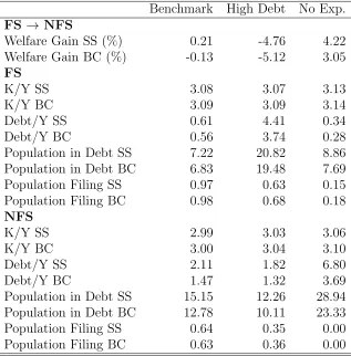
Table 4reports the welfare gain of implementing NFS along with other statistics for FS and NFS. Given how this calibration changes borrowing limits, it should not be surprising that welfare of NFS relative to FS is now much lower. Without aggregate risk, the welfare gain of moving from FS to NFS is -4.76%, i.e. a large welfare loss. With aggregate risk, the welfare gain is even lower at -5.12%. The mechanism by which it is lower is the same as in the main text: High default costs result in a contraction in credit, and NFS’ contraction is larger than FS’.
C.2
No Expenditure Shocks
Statistic Data Model Parameter Value
Targeted Statistics
Capital-Output Ratio 3.08 3.07 β 0.956
Debt-Output Ratio×100∗ 6.22 4.41 χ0 0.974
Population Filing (%) 0.93 0.63 χ1 0.563
Population in Debt (%) 17.6 20.8 πrl 0.213
Earnings Share of Top 20% 60.2 59.7 u 0.454
Earnings Mean/Median 1.57 1.84 u 27.95
Wealth Mean/Median 4.03 4.00 ξ 0.183
Untargeted Statistics
Wealth Share of Top 20% 81.7 73.0 Wealth Share of 4th Quintile 12.2 22.0 Wealth Share of 3rd Quintile 5.0 5.8 Wealth Share of 2nd Quintile 1.3 0.5
Wealth Gini 0.80 0.73
Earnings Share of 4th Quintile 22.9 16.3 Earnings Share of 3rd Quintile 13.0 11.1 Earnings Share of 2nd Quintile 4.0 7.6
Earnings Gini 0.61 0.54
Average Interest on Debt (%) 12.7 4.1 Discharged Debt-Output Ratio×100∗ 0.32 0.31 Discharged −a-Output Ratio×100∗ 0.32 0.07
Debt-Income of Filers 1.62 2.08
Debt-Income of Below Median Filers 1.66 2.10 Debt-Income of Above Median Filers 1.58 1.98 Percentage of Filers Below Median 68.8 90.7 Population withd= 1, any h (%) 0.77 Right-tail Population Filing 0.00 Right-tail Debt-Output Ratio×100 0.93
Note: Model debt is measured as −a+x, a filing is measured ash= 0 and
d= 1, and discharged debt is−a+x when h= 0 andd= 1. Statistics marked with ∗ have debt in the data measured with revolving consumer credit.
20 30 40 50 60 70 80 0
0.5 1 1.5 2 2.5 3 3.5
Age
Debt Limit
Borrowing Limits By Age
FS BC FS SS NFS BC NFS SS
Figure 3: Average Borrowing Limits by Age for a High Debt Calibration
expenditure shocks. All other parameters are kept at their baseline values.12 Note that NFS without expenditure shocks now completely eliminates default, and the model reduces to a standard incomplete markets environment with a natural borrowing limit.
Table 4reports statistics and welfare without expenditure shocks. Note that the welfare gain of moving from FS to NFS is now very large but is significantly reduced once aggregate risk is added. There is a similar story with the debt statistics where the debt-output ratio in NFS falls by 45% once aggregate risk is added. These results suggest that the levels of the welfare gain and debt associated with NFS are not robust, but how aggregate risk affects them is.
C.3
Guaranteed Earnings Prior to Retirement
While in most studies the use of a natural borrowing limit rather than some exogenously fixed limit is of secondary importance, here a natural limit occurs as the consequence of implementing NFS. Consequently, it is extremely important. There are then three issues
12 An earlier version of this paper (available by request) has no expenditure shocks in the baseline. The
Benchmark High Debt No Exp.
FS→ NFS
Welfare Gain SS (%) 0.21 -4.76 4.22
Welfare Gain BC (%) -0.13 -5.12 3.05
FS
K/Y SS 3.08 3.07 3.13
K/Y BC 3.09 3.09 3.14
Debt/Y SS 0.61 4.41 0.34
Debt/Y BC 0.56 3.74 0.28
Population in Debt SS 7.22 20.82 8.86 Population in Debt BC 6.83 19.48 7.69
Population Filing SS 0.97 0.63 0.15
Population Filing BC 0.98 0.68 0.18
NFS
K/Y SS 2.99 3.03 3.06
K/Y BC 3.00 3.04 3.10
Debt/Y SS 2.11 1.82 6.80
Debt/Y BC 1.47 1.32 3.69
Population in Debt SS 15.15 12.26 28.94 Population in Debt BC 12.78 10.11 23.33
Population Filing SS 0.64 0.35 0.00
Population Filing BC 0.63 0.36 0.00
Table 4: Robustness to Calibrations and Expenditure Shocks
to consider, namely, what is the limit in the theory, in the computation, and in the data. In the theory, the use of a log-efficiency process implies efficiency, and hence labor income, can be arbitrarily close to zero prior to retirement. However, because some labor income is guaranteed in retirement, the natural limit will not be zero as long as κG > 0. In the
computation, the log process is discretized using a large support.13 This makes the lowest efficiency realization prior to retirement close to zero. Lastly,Carroll(1992) documents that non-capital household income in the data, including transfer income, falls to (or very close to) zero between .30% and .65% of the time for working-age households.
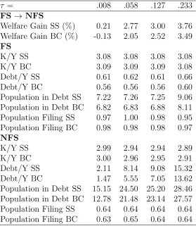
While a low minimum value for earnings during working life is thus reasonable to use, I explore the robustness of the results to this assumption by guaranteeing larger earnings. Specifically, given the efficiency distribution of the benchmark economy, I replace any values less than a threshold τ with τ and re-normalize so that N = 1 in steady state. I consider 4 different thresholds τ ∈ {.008, .058, .127, .233}. These represent a lower bound of roughly
13Specifically, the support is±6.25¯σ η,1/
p
1−¯γ2for the persistent shock and±5¯σ
εfor the transitory shock
$500, $3500, $7,600, and $14,000 taking average household labor income to be $60,000 and are the values considered in Athreya (2008).
τ = .008 .058 .127 .233
FS →NFS
Welfare Gain SS (%) 0.21 2.77 3.00 3.76 Welfare Gain BC (%) -0.13 2.05 2.52 3.49
FS
K/Y SS 3.08 3.08 3.08 3.08
K/Y BC 3.09 3.09 3.09 3.08
Debt/Y SS 0.61 0.62 0.61 0.66
Debt/Y BC 0.56 0.56 0.56 0.60
Population in Debt SS 7.22 7.26 7.25 9.06 Population in Debt BC 6.82 6.83 6.88 8.11 Population Filing SS 0.97 1.00 0.98 0.95 Population Filing BC 0.98 0.98 0.98 0.97
NFS
K/Y SS 2.99 2.94 2.94 2.89
K/Y BC 3.00 2.96 2.95 2.91
Debt/Y SS 2.11 8.14 9.08 15.32
Debt/Y BC 1.47 5.55 7.05 13.62
Population in Debt SS 15.15 24.50 25.20 28.46 Population in Debt BC 12.78 21.48 23.14 27.57 Population Filing SS 0.64 0.64 0.64 0.64 Population Filing BC 0.63 0.65 0.64 0.64
Table 5: Robustness to Guaranteed Income
Table 5reports the results. As τ increases, so does the welfare and debt associated with NFS. In contrast, FS’ statistics are virtually unchanged. However, for all the τ considered, the welfare gain and debt associated with NFS fall when aggregate risk is added.
C.4
Retirement Schemes
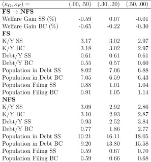
In the benchmark calibration, labor income in retirement is comprised of a guaranteed frac-tion κG=.15 of average earnings and a fractionκF =.35 of earnings from the last period of
working life. The average replacement rate is roughly 50% because κG+κF =.5. However,
as already discussed, it is not the replacement rate that really matters but how much of it is guaranteed. I now examine the robustness of the results to alternative replacement schemes (κG, κF) subject to keeping κG+κF =.5.
(κG, κF) = (.00, .50) (.30, .20) (.50, .00)
FS → NFS
Welfare Gain SS (%) -0.59 0.07 -0.01 Welfare Gain BC (%) -0.65 -0.22 -0.30
FS
K/Y SS 3.17 3.02 2.97
K/Y BC 3.18 3.02 2.97
Debt/Y SS 0.61 0.61 0.61
Debt/Y BC 0.55 0.57 0.60
Population in Debt SS 8.02 7.06 6.88 Population in Debt BC 7.05 6.59 6.43 Population Filing SS 0.88 1.01 1.04 Population Filing BC 0.91 1.05 1.14
NFS
K/Y SS 3.09 2.92 2.86
K/Y BC 3.10 2.93 2.87
Debt/Y SS 0.93 2.52 3.84
Debt/Y BC 0.77 1.86 2.77
Population in Debt SS 10.21 16.11 18.05 Population in Debt BC 9.20 13.80 15.58 Population Filing SS 0.59 0.67 0.70 Population Filing BC 0.59 0.66 0.68
Table 6: Robustness of Results to Alternative Retirement Schemes
Table 6 records the results. Overall, welfare in levels is not greatly affected by these changes. Also, in each case aggregate risk causes the welfare and debt associated with NFS to fall with the largest reductions in debt occurring forκG =.5. These results agree with the
References
K. B. Athreya. Default, insurance and debt over the life-cycle. Journal of Monetary Eco-nomics, 55(4):752–774, 2008.
G. Bermant and E. Flynn. Incomes, debts, and repayment capacities of recently discharged chapter 7 debtors.http://www.justice.gov/ust/eo/public_affairs/articles/docs/
ch7trends-01.htm, Jan. 1999. Accessed: October 27, 2014.
C. D. Carroll. The buffer-stock theory of saving: Some macroeconomic evidence. Brookings Papers on Economic Activity, 23(2):61–156, 1992.
S. Chatterjee, D. Corbae, M. Nakajima, and J.-V. R´ıos-Rull. A quantitative theory of unsecured consumer credit with risk of default. Econometrica, 75(6):1525–1589, 2007.
J. Fern´andez-Villaverde and D. Krueger. Consumption over the life cycle: Facts from the consumer expenditure survey data. The Review of Economics and Statistics, 89(3):552– 565, 2007.
R. G. Hubbard, J. Skinner, and S. P. Zeldes. The importance of precautionary motives in explaining individual and aggregate saving. Carnegie-Rochester Conference Series on Public Policy, 40(1):59–125, 1994.
F. Karahan and S. Ozkan. On the persistence of income shocks over the life cycle: Evidence and implications. PIER Working Paper 11-030, University of Pennsylvania, 2011.
P. Krusell and A. A. Smith, Jr. Income and wealth heterogeneity in the macroeconomy.
Journal of Political Economy, 106(5):867–896, 1998.
I. Livshits, J. MacGee, and M. Tertilt. Consumer bankruptcy: a fresh start. American Economic Review, 97(1):402–418, 2007.
I. Livshits, J. MacGee, and M. Tertilt. Accounting for the rise in consumer bankruptcies.
American Economic Journal: Macroeconomics, 2(2):165–93, 2010.
L. Ohanian and A. Raffo. Hours worked over the business cycle in OECD countries, 1960-2010. Mimeo, 2011.
G. Tauchen. Finite state Markov-chain approximations to univariate and vector autoregres-sions. Economics Letters, 20(2):177–181, 1986.
E. N. Wolff. Recent trends in household wealth in the united states: Rising debt and the middle-class squeeze—an update to 2007. Working Paper 589, Levy Economics Institute of Bard College, 2010.