Download Download PDF

(1)

PREDICTING WATER LEVELS AT KAINJI DAM USING

ARTIFICIAL NEURAL NETWORKS

C.C. Nwobi-Okoyea, A.C. Igboanugob

a

Emeagwali Centre for Research, Anambra State University, Uli, Anambra State, Nigeria.

Emails: [email protected], [email protected]

b

Department of Production Engineering, University of Benin, Benin City, Edo State, Nigeria.

Email: [email protected]

Abstract

Poor electricity generation in Nigeria is a very serious problem. Accurate prediction of water levels in dams is very important in power planning. Effective power planning helps in ensuring steady supply of electric power to consumers. The aim of this study is to develop artificial neural network models for predicting water levels at Kainji Dam, which supplies water to Nigeria’s largest hydropower generation station. It involves taking of a ten-year record of the daily water levels at the dam from 2001 to 2010. The daily water level data were used to develop five neural network models and an Autoregressive Integrated Moving Average (ARIMA) model to fit the daily water levels obtained in the year 2010. The results show that the prediction accuracy of the neural network models increased with increasing input, but after the four-input model the accuracy started declining. The four-input neural network model had the lowest relative error of 0.062 percent while the single-input model had the highest relative error of 0.237 percent. The ARIMA model with relative error of 0.039 percent had the best prediction. Generally, the models’ predictions were good, but the neural network models which involve little mathematics were much simpler to build. The developed models will be very useful in power planning in Nigeria’s hydropower stations for more efficient power supply.

Keywords: artificial neural network, hydropower, ARIMA, time series, modelling

1. Introduction

Poor electric power generation and supply has re-mained a very serious problem in Nigeria ever since the 80s. The problem has hampered industrial devel-opment and contributed immensely to the poor eco-nomic state of Nigeria. Improving power generation in Nigeria has been a top priority of successive Nige-rian government since 1999. Apart from insufficient number of power generation plants, existing ones are facing declining output due to ageing, neglect, ineffec-tive maintenance and inefficient management [1].

Water levels determine the power outputs in dams. The variations in water level lead to variations in wa-ter flow across the wawa-ter turbines which generate elec-tricity and consequent variation in electric power out-puts from the generators [1]. Hence, accurate predic-tion of water levels in dams is very important in gen-eration planning. Proper and effective power planning helps in ensuring steady supply of electrical power to consumers. Improved electric power supply to

con-sumers will lead to increase in gross domestic product of the country and better standard of living for the populace.

Water level variations are a time series. National In-stitute of Standards and Technology [2] defined time series as an ordered sequence of values of a variable at equally spaced time intervals. Time series is very im-portant and ubiquitous in our daily lives. As noted by Cryer and Chan [3], the purpose of time series anal-ysis is generally twofold: to understand or model the stochastic mechanism that gives rise to an observed series and to predict or forecast the future values of a series based on the history of that series and, possibly, other related series or factors. For detailed literature on time series analysis see ([4], [5], [6] and [7]). One area of application of neural networks is in time series prediction.

(2)

net-works [8]. The concept of artificial neurons was first introduced in 1943 by McCulloch and Pitts [9]. Rus-sell and Norvig [8] stated that since 1943 when Mc-Culloch and Pitts introduced the concept of neurons, much more detailed and realistic models have been developed both for neurons and for larger systems in the brain leading to the modern field of computa-tional neuroscience. Since the work of McCulloch and Pitts in 1943, ANN has had wide application in many spheres of life. According to Maier and Dandy [10], in recent years, Artificial Neural Networks (ANNs) have become extremely popular for prediction and forecast-ing in a number of areas, includforecast-ing finance, power gen-eration, medicine, water resources and environmental science.

The utility of artificial neural network models lies in the fact that they can be used to infer a function from observations. This is particularly useful in ap-plications where the complexity of the data or task makes the design of such a function by hand imprac-tical [8]. The tasks to which artificial neural networks are applied tend to fall within the following broad cat-egories:

Function approximation, or regression analysis, including time series prediction, fitness approxi-mation and modelling.

Classification, including pattern and sequence recognition, novelty detection and sequential de-cision making.

Data processing, including filtering, clustering, blind source separation and compression.

Robotics, including directing manipulators, Com-puter numerical control.

Many papers have been written on the application of ANNs to time series analysis. Kuligowski and Bar-ros [11] in their paper described a simple precipitation forecasting model based on artificial neural networks. Their model used the radiosonde-based 700-hPa wind direction and antecedent precipitation data from a rain gauge network to generate short-term (06 h) pre-cipitation forecasts for a target location. Guh and Hsieh [12] in their paper proposed an artificial neu-ral network based model, which contains seveneu-ral back propagation networks, to both recognize the abnormal control chart patterns and estimate the parameters of abnormal patterns such as shift magnitude, trend slope, cycle amplitude and cycle length, so that the manufacturing process can be improved. Their nu-merical results showed that the proposed model also has a good recognition performance for mixed abnor-mal control chart patterns

Maier and Dandy [10] reviewed 43 papers dealing with the use of neural network models for the pre-diction and forecasting of water resources variables in

terms of the modelling process adopted. They iden-tified inadequate model building as the obstacle mili-tating against accurate predictions using artificial net-works. They suggested that ANN models must be properly evaluated before its application in time se-ries analysis. Their assertion is corroborated by Chat-field (1993) when commenting on the suitability of ANNs for time series analysis and forecasting, who commented thus: “when the dust has settled, it is usu-ally found that the new technique is neither a mirac-ulous cure-all nor a complete disaster, but rather an addition to the analyst’s toolkit which works well in some situations and not in others”.

It is important to note that a neural network mod-elling is purely a computational technique. Hence, if one wants to explain an underlying process or math-ematical framework that produces the relationships between the dependent and independent variables, it would be better to use a more traditional statistical model. However, if model interpretability is not im-portant, one can often obtain good model results more quickly using a neural network.

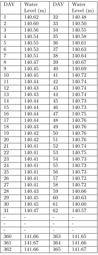
The hub of our investigation is the Kainji Dam of Kainji Hydro Electric Power PLC, which with an in-stalled capacity of 760MW [1], is Nigerias largest hy-dropower station. A ten-year (2001 to 2010) daily water level data were obtained and some of these are depicted in Table 1 for the year 2010. Kainji Dam was built in 1969 across the River Niger on Kainji Island, to impound water to generate Electricity. The height of the dam from its toe to the crest is 65.5m (215ft). The length is 8.04 kilometers. In compliance with the interntional law on dams across international rivers, Kainji dam has two navigational locks.the Upper and Lower locks. These locks are opened for the passage of barges or boats from the upstream to the down stream of the dam.

The dam construction caused the formation of a lake known as Kainji Lake. The lake acts as a reser-voir for the dam. The lake has two flooding seasons, namely the white and black floods. The white flood is the inflow of flood into the reservoir, from rains within the catchment areas of the river within Nigeria. On the other hand, the Black flood is the inflow of flood into the reservoir from rains in the catchment areas of the river outside Nigeria, e g Guinea, Mali, Niger, etc. The White flood arrives the lake in around the month of July since its journey to the lake is not far. The Black flood arrives in December as it has to travel long distance from those countries mentioned above.

(3)

ANN Prediction of Water Levels at Kainji Dam

Table 1: Table of daily water level in 2010.

DAY Water Level (m)

DAY Water Level (m) 1 140.62 32 140.48 2 140.60 33 140.50 3 140.56 34 140.55 4 140.54 35 140.58 5 140.55 36 140.61 6 140.53 37 140.63 7 140.51 38 140.64 8 140.47 39 140.67 9 140.45 40 140.69 10 140.45 41 140.72 11 140.44 42 140.74 12 140.43 43 140.74 13 140.43 44 140.74 14 140.44 45 140.73 15 140.44 46 140.73 16 140.44 47 140.75 17 140.44 48 140.76 18 140.43 49 140.76 19 140.42 50 140.76 20 140.42 51 140.76 21 140.41 52 140.74 22 140.41 53 140.75 23 140.41 54 140.73 24 140.41 55 140.73 25 140.41 56 140.73 26 140.41 57 140.72 27 140.41 58 140.72 28 140.43 59 140.66 29 140.45 60 140.63 30 140.45 61 140.60 31 140.47 62 140.57

- - -

-- - -

-360 141.66 363 141.65 361 141.67 364 141.66 362 141.66 365 141.67

(3.0000×109 m3_{) constitute the dead storage, ie} wa-ter below the level of the penstock. The remaining 12 Billion (12.0000×109m3_{) constitute the life or usable} storage.

Neural network approach was used to predict the water levels of Kainji dam water reservoir. Water level prediction is necessary in power planning at the hydropower station. The neural network model de-veloped has intuitive and theoretical appeal. It was developed based on the assumption that the time se-ries was generated by a stochastic process.

2. Methodology

A 10-year daily water level data were obtained from Kainji Hydroelectric Power Company PLC, Kainji, New Bussa, Niger State, Nigeria. The data were used to forecast the daily water levels using Box-Jenkins’s times series modelling methodology and artificial neu-ral network model.

2.1. Time series modelling methodology

In time series analysis, an autoregressive model is represented in the following form (Box et al. (1994), Casella et al (2006), Cryer and Chan (2008)).

xt=φ1xt−1+φ2xt−2+· · ·+φp+xt−p+ωt (1)

Similarly, a moving average model is represented in the following form (Box et al. (1994), Casella et al (2006), Cryer and Chan (2008)).

xt=ωt+θ1ωt−1+θ2ωt−2+· · ·+θqωt−q (2)

Autoregressive Integrated Moving Average Model (ARIMA) was pioneered by the land mark work of Box and Jenkins (1970); hence it is often referred to as Box-Jenkins method. This model integrates the autoregressive and moving average models with ap-propriate differencing to achieve stationarity. In or-der words, ARIMA extends the combination of AR and MA process to non stationary processes. From equations 1 and 2, equation (3) is obtained:

xt=θ1xt−1+· · ·+θpxt−p+ωt+θ1ωt−1+· · ·+θq+ωt−q (3) Equation (3) could be represented in shortened form as:

φ(B)xt=θ(B)ωt (4)

If the output xt is differenced dtimes to achieve sta-tionarity, equation 5 is obtained.

∇d_x

t= (1−B)dxt (5)

In general by combining equations 4 and 5, the model could be written as:

φ(B)(1−B)dxt=θ(B)ωt (6)

(4)

Figure 1: Single input neural network model.

2.2. Neural network modelling methodology

The developed neural network models are feed for-ward multiplayer perceptron networks (MLP). The hidden units use the sigmoid activation function. As our application is for time series prediction, we used supervised learning. Seventy five (75%) percent of the data was used for training, while twenty five (25%) percent was used for testing and validation. The num-ber of epoch was set to 1000.

Five network architectures were used in the study. The first network architecture consists of single input unit, a single hidden layer with two hidden units and one output unit, the second network architecture con-sists of two input units, a single hidden layer with two hidden units and one output unit, the third network architecture consists of three input units, a single hid-den layer with three hidhid-den units and one output unit, the fourth network architecture consists of four input units, a single hidden layer with four hidden units and one output unit while the fifth network architecture consists of five input units, a single hidden layer with five hidden units and one output unit.

Given an input vector (X = (x1, x2)), the activa-tions of the input units are set to (a1, a2) = (x1, x2) and the network computes to:

Ini = n

X

j=1

Wj,iaj (7)

ai =g(Ini) (8)

For the single input network shown in Figure 1, the network computes to:

a4=g(W2,4a2+W3,4a3) (9)

a4=g(W2,4g(W1,2a1) +W3,4g(W1,3a1)) (10)

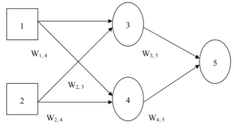
For the two-input network shown in Figure 2, the network computes to:

a5=g(W3,5a3+W4,5a4) (11)

a5=g(W3,5g(W1,3a1+W2,3a2)+W4,5g(W1,4a1+W2,4a2)) (12)

Figure 2: Two-input neural network model.

For the single input architecture, the input vec-tor is X = (Xt−367), for the two input

architec-ture, the input vector is X = (Xt−367, Xt−732),

for the three input architecture in Figure 3, the input vector is X = (Xt−367, Xt−732, X1097), for the four input architecture, the input vec-tor is X = (Xt−367, Xt−732, X1097, Xt−1463) while for the five input architecture, the input vector is X = (Xt−367, Xt−732, Xt−1097, Xt−1463, Xt−1828). The learning process uses the sum of squares error criterion E to measure the effectiveness of the learn-ing algorithm.

E=Err2≡(Xt−hW(x))2 (13)

Here

b

Xt=hW(x) (14)

hW(x) is the output of the perceptron.

3. Results

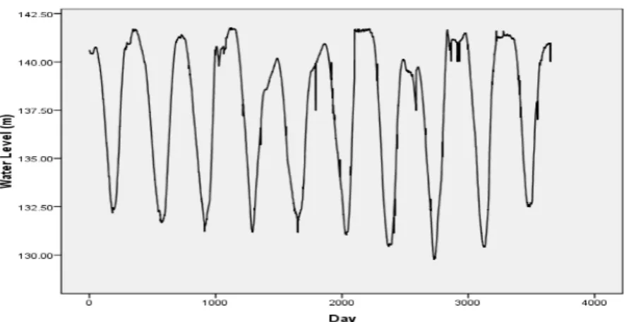
Table 1 shows part of the 10-year data obtained from Kainji Hydropower PLC, the graph of the water level variations from the year 2001 to 2010 is shown in Figure 4.

(5)

Figure 3: Three-input neural network model.

(6)

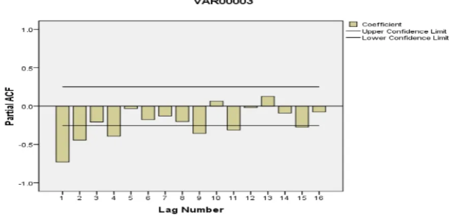
Figure 5: ACF of the water level series.

river show marked effect in the dry season of Nigeria which occurs in November, December, January and February. Then it starts ebbing.

Analysing the water level series, stationarity was obtained after first differencing. Examination of the ACF and PACF in Figures 5 and 6 show that there are two significant ACF and PACF at lag 1 and 2 with the ACF values being -0.728 and 0.322 respectively. The negative values of the significant ACF and PACF are indicative that moving average two (MA (2)) model with the coefficients θ1>0 andθ2>0 respectively is the appropriate model to use.

According to Shumway and Stoffer [7], for MA (q) model we have:

ρ(h) =

Pq−h

j=0θjθj+h 1 +θ2

1+· · ·+θq2

(15)

Butq= 2 and ifh= 1 we have:

Substituting the first significant value of the ACF we obtain

ρ(1) =θ0θ1+θ1θ2 1 +θ2

1+θ 2 2

=−0.728 (16)

Similarly, if h = 2 we have:

ρ(2) =

P0

j=0θjθj+2 1 +θ2

1+θ22

(17)

And for

ρ(h) =ρ(2) = θ0θ2 1 +θ2

1+θ22

= 0.322 (18)

ρ(1) ρ(2) =

θ0θ1+θ1θ2 θ0θ2

= 2.261 (19)

But θ0 = 1. This is because for moving average 2 (MA 2) models, the coefficient θ0 = 1 see [5] and [7]. Hence,θ2=θ1+θ1θ2

Letθ2=−0.2,θ2 was chosen to be 0.2 because for moving average 2 (MA 2) models whereρ(1)<0 and whose patterns correspond to Figures 6 and 7, the coefficientsθ2 andθ1must be greater than 0 and less than 1. This is because of the bounds of invertibility conditions (see [5] pages 307 and 310, and [7]). Hence, θ1= 0.56525.

Fitting the coefficients θ2 and θ1 into the formula for MA 2 models [4, 5 and 7] equation (18) is obtained.

xt=et−θ1et−1+θ2et−2 (20)

xt=et−0.56525et−1+ 0.2et−2

But

Xt−Xt−366=xt (21)

xt−xt−1=St (22)

St=et−θ1et−1+θ2et−2 (23)

et=St+θ1et−1+θ2et−2 (24)

et=αt (25)

αt=St+θ1et−1+θ2et−2 (26)

In forecasting form:

xt=xt−1−θ1et−1+θ2et−2 (27)

Substituting equation (25) into (19), equation (26) is obtained.

(7)

Figure 6: PACF of the water level series.

Table 2: Model type vs errors.

Description Sum of

Squares Error

Relative Error(%) Single input neural

network model

60.189 0.237

Two input neural network model

26.505 0.104

Three input neural network model

26.028 0.089

Four input neural network model

16.310 0.062

Five input neural network model

18.230 0.065

ARIMA model 2.732 0.039

b

Xt=Xt−366+xt−1−56525et−1+ 0.2et−2 (29)

A comparison of the results of fitting the ARIMA and neural network models to water levels data in the year 2010 is shown in Table 2.

4. Discussion

Examining Table 2 above shows that as the number of inputs to the neural network increased, the sum of squares error and the relative error decreased. This increase continued until the input reached four. Af-ter the four input architecture, the errors started in-creasing. Generally, the sum of squares error and the relative error of the ARIMA model at values of 2.732 and 0.039 respectively was lower than the minimum obtained from the neural network models which are 16.310 and 0.062 respectively. Hence, in this

partic-ular case study, the ARIMA model predicted better than the neural network models.

The decrease in prediction error of the neural net-work with increasing number of inputs could be at-tributed to the fact that as the more the inputs, the more the learning experience of the network. But at a certain number of inputs, the experience no longer counts in network performance. This could be due to the fact that the experience became old and obsolete, and was no longer relevant in the current situation. The variations in the sum of squares error and the relative error of the neural network confirm the fact that the performance of the network depends on the network design architecture ([10], [13]).

Generally, the neural network models were bereft of the messy mathematics and statistical analysis re-quired in building the ARIMA model, while at the same time giving good model predictions. Hence, would be preferable when the underlying mathemat-ical structure behind the model predictions is irrele-vant to the modeller/analyst, and model building is required quickly.

Hydrological prediction is not only important in en-vironmental studies [14], but as earlier noted very nec-essary in power generation planning. Generation plan-ning and performance evaluation is very important in electric power generation and distribution systems [1, 15, 16 and 17]. It is obvious that neural network mod-els will help in efficient power planning.

5. Conclusion

(8)

desirable [18, 19 and 20]. Electricity power supply acts as an engine that drives an economy. Sufficient power supply is very vital for industrial development and economic growth of any nation. The authorities in Nigeria as part of their effort to reform the power sector in the country set benchmark for performance evaluation of power generation, transmission and dis-tribution facilities. Chief Executive Officers of Power companies that failed to meet the minimum bench-mark requirements were sacked by the government [20]. We have successfully developed in this paper a very sound and statistically robust methods and mod-els in aid of power planning of hydropower plants. It is suggested that the authorities in Nigeria and else-where adopt this research for power planning of hy-dropower generation facilities.

Finally, if the recommendations of this research are implemented by adopting this novel power planning aid and making sure hydropower generation stations stick to it. There will be resultant improvement in the operations of the power stations, with attendant im-provement in power supply in Nigeria and elsewhere. This will have a very positive effect on the state of Nigerias economy which has been declining over the years. The same applies to other countries that are in similar situation as Nigeria.

Acknowledgement

The assistance rendered by the management of Kainji Hydro Electricity Plc, New Bussa, Niger State, Nigeria is hereby acknowledged.

References

1. Nwobi-Okoye, C.C. and Igboanugo, A.C. Perfor-mance Evaluation of Hydropower Generation System Using Transfer Function Modelling. International Journal of Electrical Power and Energy Systems, 45 (1), pp245254, 2012.

2. National Institute of Standards and Technology.

NIST/SEMATECH e-Handbook of Statistical Meth-ods. NIST, US Commerce Department, USA (2010). Available from: http://www.itl.nist.gov/div898/ handbook/. [Assessed 4th August 2010].

3. Cryer, J.D. and Chan, K.Time Series Analysis with Applications in R. Springer Science+Business Media, LLC, 233 Spring Street, New York, NY 10013, USA, 2008.

4. Box, G.E.P., Jenkins, G.M. and Reinsel, G.C.Time Series Analysis Forecasting and Control. McGraw-Hill Inc., USA, 1994.

5. DeLurgio, S.A. Forecasting Principles and Applica-tions. 3rd Edn, McGraw-Hill, New York, USA, 1998. 6. Igboanugo, A.C. and Nwobi-Okoye, C.C. Production Process Capability Measurement and Quality Control Using Transfer Functions. Journal of the Nigerian Association of Mathematical Physics, 19(1), 2011, 453-464.

7. Shumway, R. H. and Stoffer, D.S. Time Series Analysis and Its Applications in R. Springer Sci-ence+Business Media, LLC, 233 Spring Street, New York, NY 10013, USA, 2006.

8. Russell, S.J. and Norvig, P.Artificial Intelligence: a modern approach. Pearson Educational Inc., Upper Saddle River, New Jersey, USA, 2003.

9. McCulloch, W.S. and Pitts, W. A logical calculus of the ideas imminent in nervous activity. Bulletin and Mathematical Biophysics, 5, 1943, pp115–133. 10. Maier, H.R. and Dandy G.C. Neural networks for the

prediction and forecasting of water resources vari-ables: a review of modelling issues and applica-tions. Environmental Modelling & Software, 15, 2000, pp101–124.

11. Kuligowski, Robert J., Barros Ana P. Experiments in Short-Term Precipitation Forecasting Using Artifi-cial Neural Networks. Monthly Weather Review, 126, 1998, pp470–482.

12. Guh, R. and Hsieh, Y. A neural network based model for abnormal pattern recognition of control charts.

Computers & Industrial Engineering, 36(1), 1999, pp97–108.

13. Chatfield, C. Neural networks: Forecasting break-through or just a passing fad? International Journal of Forecasting, 9, 1993, pp 1–3.

14. Folly, K.A. Performance evaluation of power system stabilizers based on Population-Based Incremental Learning (PBIL) Algorithm. Int. Journal of Elec-trical Power and Energy Systems, 33 (7), 2011, pp 1279–1287.

15. Jyothsna, T.R. and Vaisakh, K. Design and perfor-mance evaluation of SSSC supplementary modulation controller in power systems using SPEF method. Int. Journal of Electrical Power and Energy Systems, 35 (1), 2012, pp158–170.

16. Ghedamsi, K. and Aouzellag, D. Improvement of the performances for wind energy conversions systems.

Int. Journal of Electrical Power and Energy Systems, 32 (6), 2010, pp936–945.

17. de Sousa, M. P. A., Manoel Ribeiro Filho, Marcus Vin´ıcius Alves Nunes and Andrey da Costa Lopes, Maintenance and operation of a hydroelectric unit of energy in a power system using virtual reality. Int. Journal of Electrical Power and Energy Systems, 32 (6), 2010, pp599–606.

18. Zhang, Y., Wang, Z., Zhang, J. and Ma, J. Fault localization in electrical power systems: A pattern recognition approach. Int. Journal of Electrical Power and Energy Systems, 33 (3), 2011, 791–798. 19. Nnaji sacks four PHCN executives. Nigerian Daily