O R I G I N A L R E S E A R C H
Open Access
Iterative algorithm for the reflexive solutions
of the generalized Sylvester matrix equation
Mohamed A. Ramadan, Naglaa M. El
–
shazly
*and Basem I. Selim
* Correspondence:naglaamoh1@ yahoo.com
Department of Mathematics and Computer Science, Faculty of Science, Menoufia University, Shebein El-Koom, Egypt
Abstract
In this paper, the generalized Sylvester matrix equationAV+BW=EVF+Cover reflexive matrices is considered. An iterative algorithm for obtaining reflexive solutions of this matrix equation is introduced. When this matrix equation is consistent over reflexive solutions then for any initial reflexive matrix, the solution can be obtained within finite iteration steps. Furthermore, the complexity and the convergence analysis for the proposed algorithm are given. The least Frobenius norm reflexive solutions can also be obtained when special initial reflexive matrices are chosen. Finally, numerical examples are given to illustrate the effectiveness of the proposed algorithm.
Keywords:Generalized Sylvester matrix equation, Iterative method, Reflexive matrices, Least Frobenius norm solution
2010 Mathematics Subject Classification:15A06, 65F10, 65F30
Introduction and preliminaries
Consider the generalized Sylvester matrix equation
AVþBW ¼EVFþC; ð1:1Þ
where A, E∈Rm×p, B∈Rm×q,F∈Rn×n, andC∈Rm×nwhile V∈Rp×nandW∈Rq×n are matrices to be determined. Ann×nreal matrixP∈Rn×nis called a generalized reflection matrix ifPT=PandP2=I. Ann×nmatrixAis said to be reflexive matrix with respect to the generalized reflection matrixPifA=PAPfor more details see [1,2]. The symbolA⊗B stands for the Kronecker product of matricesAandB. The vectorization of anm×nmatrix A, denoted byvec(A), is themn× 1 column vector obtains by stacking the columns of the matrixAon top of one another: vecðAÞ ¼ ðaT
1 aT2…aTnÞ T
. We usetr(A) andATto denote the trace and the transpose of the matrix Arespectively. In addition, we define the inner product of two matricesA,Bas〈A,B〉=tr(BTA). Then, the matrix norm ofAinduced by this inner product is Frobenius norm and denoted by‖A‖where〈A,A〉=‖A‖2.
The reflexive matrices with respect to the generalized reflection matrixP∈Rn×nhave many special properties and widely used in engineering and scientific computations [2,3]. Several authors have studied the reflexive solutions of different forms of linear matrix equations; see for example [4–7]. Ramadan et al. [8] considered explicit and iterative methods for solving the generalized Sylvester matrix equation. Dehghan and Hajarian [9] constructed an iterative algo-rithm to solve the generalized coupled Sylvester matrix equations (AY−ZB,CY−ZD) = (E,F) over reflexive matrices. Also, Dehghan and Hajarian [10] proposed three iterative
algorithms for solving the linear matrix equation A1X1B1+A2X2B2=C over reflex-ive (anti -reflexreflex-ive) matrices. Yin et al. [11] presented an iterative algorithm to solve
the general coupled matrix equations P j¼1 q
AijXjBij¼Miði¼1;2;⋯;pÞ and their optimal
approximation problem over generalized reflexive matrices. Li [12] presented an iterative algorithm for obtaining the generalized (P,Q)-reflexive solution of a
quaternion matrix equation P l¼1 u
AlXBlþ
Pv
s¼1CsXD~ s¼ F. In [13], Dong and Wang presented necessary and sufficient conditions for the existence of the {P,Q,k+ 1}-reflexive (anti-reflexive) solution to the system of matricesAX=C,XB=D. In [14], Nacevska found necessary and sufficient conditions for the generalized reflexive and anti-reflexive solution for a system of equations ax=b andxc=din a ring with involution. Moreover, Hajarian [15] established the matrix form of the biconjugate residual (BCR) algorithm for computing the generalized reflexive (anti-reflexive) solutions of the generalized Sylvester matrix equation
P
i¼1 s
AiXBiþ
Pt
j¼1CjYDj¼M. Liu [16] established some conditions for the existence and the representations for the Hermitian reflexive, anti-reflexive, and non-negative definite reflexive solutions to the matrix equationAX=Bwith respect to a generalized reflection
P by using the Moore-Penrose inverse. Dehghan and Shirilord [17] presented a generalized MHSS approach for solving large sparse Sylvester equation with non-Hermitian and complex symmetric positive definite/semi-definite matrices based on the MHSS method. Dehghan and Hajarian [18] proposed two algorithms for solving the generalized coupled Sylvester matrix equations over reflexive and anti-reflexive matrices. Dehghan and Hajarian [19] estab-lished two iterative algorithms for solving the system of generalized Sylvester matrix equa-tions over the generalized bisymmetric and skew-symmetric matrices. Hajarian and Dehghan [20] established two gradient iterative methods extending the Jacobi and Gauss Seidel iter-ation for solving the generalized Sylvester-conjugate matrix equiter-ation A1XB1+A2XB2+ C1YD1+C2YD2=E over reflexive and Hermitian reflexive matrices. Dehghan and Hajarian [21] proposed two iterative algorithms for finding the Hermitian reflexive and skew– Hermit-ian solutions of the Sylvester matrix equationAX+XB=C. Hajarian [22] obtained an iterative algorithm for solving the coupled Sylvester-like matrix equations. El–Shazly [23] studied the
perturbation estimates of the maximal solution for the matrix equationXþATpffiffiffiffiffiffiffiffiX−1A¼P. Khader [24] presented numerical method for solving fractional Riccatidifferential equation
(FRDE). Balaji [25] presented a Legendre wavelet operational matrix method for solving the nonlinear fractional order Riccati differential equation. The generalized Sylvester matrix equa-tion has numerous applicaequa-tions in control theory, signal processing, filtering, model reducequa-tion, and decoupling techniques for ordinary and partial differential equations (see [26–29]).
Iterative algorithm for solvingAV+BW=EVF+C In this part, we consider the following problem:
Problem 2.1. For given matricesA,B,E,C∈Rm×n,F∈Rn×n, and two generalized reflec-tion MatricesP,Sof sizen, find the matricesV∈Rnn
r ðPÞandW∈Rn
n
r ðSÞsuch that
AVþBW ¼EVFþC ð2:1Þ
Where the subspaceRnrnðPÞis defined byRnrnðPÞ ¼ fQ∈Rnn:Q¼PQPg, wherePis the generalized reflection matrix:P2=I,PT=P.
An iterative algorithm for solving the consistent Problem 2.1
In the next theorem, we prove that the solutions {Vk+ 1} and {Wk+ 1} are reflexive solutions for the matrix Eq. (2.1).
Theorem 2.1The solutions{Vk+ 1}and{Wk+ 1}generated from Algorithm 2.1 are reflexive solutions with respect to the generalized reflection matrices P and S of the matrix Eq. (2.1).
ProofBy using the induction we can prove this theorem as follows: Fork= 1,
PV2P¼PV1Pþ
R1
k k2
P1
k k2þ Q 1
k k2PP1P
¼V1þ
R1
k k2
P1
k k2þ Q 1
k k2
1 2 PA
TR
1PþP2ATR1P2−PETR1FTP−P2ETR1FTP2
¼V1þ
R1
k k2
P1
k k2þ Q 1
k k2
1 2 PA
TR
1PþATR1−PETR1FTP−ETR1FT
¼V2
Assume thatPVkP=Vki.e.,
PVkP¼PVk−1Pþ
Rk−1
k k2
Pk−1
k k2þ Q k−1
k k2PPk−1P¼Vk−1þ
Rk−1
k k2
Pk−1
k k2þ Q k−1
k k2Pk−1¼Vk
Now,
PVkþ1P¼PVkPþ kRkk
2
kPkk2þkQkk2PPkP ¼Vkþ kRkk
2
kPkk2þkQkk2ð
1 2½PA
TR
kPþP2ATRkP2−PETRkFTP−P2ETRkFTP2 þ kRkk
2
kRk−1k2PPk−1PÞ
¼Vkþ kRkk
2
kPkk2þkQkk2ð
1 2½PA
TR
kPþATRk−PETRkFTP−ETRkFT þkRkk
2
kRk−1k2Pk−1Þ ¼Vkþ1
Similarly, we can prove Wk+ 1 is reflexive solution with respect to the generalized reflection matrixSof the matrix Eq. (2.1).
The complexity of the proposed iterative algorithm
Algorithmic complexity is concerned about how fast or slow particular algorithm per-forms. We define complexity as a numerical function T(n)—time versus the input size
n. The complexity of an algorithm signifies the total time required by the program to run till its completion. The time complexity of algorithms is most commonly expressed using thebigOnotation. It is an asymptotic notation to represent the time complexity. A theoretical and very crude measure of efficiency is the number of floating point oper-ations (flops) needed to implement the algorithm. A “flop” is an arithmetic operation: +, x, or /. In this subsection, we compute the flops of the proposed Algorithm 2.1 of the Sylvester matrix equationAV+BW=EVF+C.
The flop counts for step 3:
The residualR1requires 4mn(2n−1) + 3mnflops, computing the reflection matrix P1 requires 4n2(2m−1) + 4n2(2n−1) + 2mn(2n−1) + 4n2flops, and computing the reflec-tion matrixQ1requires 2n2(2m−1) +n2(2n−1) +mn(2n−1) + 2n2flops.
The flop counts for step 5:
Computing Vk+ 1 requires [6n2+ 2mn+ 5] flops, Wk+ 1 requires [6n2+ 2mn+ 5] flops, Rk+ 1
requires [4mn(2n−1) + 4n2+ 6mn+ 5] flops,Qk+ 1requires [2n2(2m−1) +n2(2n−1) + mn(2n−1) + 4n2+ 4mn+ 3] flops, andPk+ 1requires [4n2(2m−1) + 3n2(2n−1) + 2mn(2n −1) + 6n2+ 4mn+ 3] flops.
k6n2ð2m−1Þ þ4n2ð2n−1Þ þ7mnð2n−1Þ þ26n2þ18mnþ21
þ6n2ð2m−1Þ þ5n2ð2n−1Þ þ7mnð2n−1Þ þ6n2þ3mn≈k12n2mþ8n3þ14mn2 þ12n2mþ10n3þ14mn2
wherekrepresents the number of iterations which is needed to find the reflexive solu-tions of Eq. (2.1). We can conclude that the total flop count of Algorithm 2.1 is O(n3).
Convergence analysis for the proposed algorithm
In this section, first, we present two lemmas which are important tools for the conver-gence of Algorithm 2.1.
Lemma 3.1 Assume that the sequences {Ri}, {Pi} and{Qi} are obtained by Algorithm
2.1, if there exists an integer number s> 1, such that Ri≠0; for all i= 1, 2,…,s,then we
have
tr RTjRi
¼0 and tr PTjPiþQTjQi
¼0;i;j¼1;2;…;s;i≠j ð3:1Þ
Proof In view of the fact thattr(Y) =tr(YT) for arbitrary matrixY. Therefore, we only need to prove that
tr RTjRi
¼0;tr PTjPiþQTjQi
¼0;for 1≤i< j≤s ð3:2Þ
We prove the conclusion (3.2) by induction through the following two steps. Step 1: First, we show that
tr RTiþ1Ri
¼0 andtr PTiþ1PiþQTiþ1Qi
¼0;i¼1;2;…;s ð3:3Þ
To prove (3.3), we also use induction.
For i= 1, noting thatP1=PP1P, andQ1=SQ1S, from the iterative Algorithm 2.1, we
can writetrðRT2R1Þ ¼trð½R1− kR1k 2
kP1k2þkQ1k2ðAP1−EP1FþBQ1Þ T
R1Þ
¼k kR1 2− k kR1 2
P1
k k2þ Q1
k k2tr P
T
1ATR1−FTPT1ETR1þQT1BTR1
¼k kR1 2− R1
k k2 P1
k k2þ Q 1
k k2tr P
T
1ATR1−PT1ETR1FTþQT1BTR1
¼k kR1 2− R1
k k2 P1
k k2þ Q1
k k2 tr P
T
1
ATR1þPATR1P−ETR1FT−PETR1FTP 2
þQT1
BTR1þSBTR1S 2
þQT1
BTR1−SBTR1S 2
þPT1
ATR1−PATR1P−ETR1FTþPETR1FTP 2
¼k kR1 2− R1
k k2 P1
k k2þ Q1
k k2 tr P
T
1 ATR
1þPATR1P−ETR1FT−PETR1FTP 2
þQT1 BTR
1þSBTR1S 2
¼k kR1 2− R1
k k2 P1
k k2þ Q1
k k2 tr P
T
1P1þQT1Q1Þ
¼0:
ð3:4Þ
tr PT
2P1þQT2Q1
¼tr A
TR
2þPATR2P−ETR2FT−PETR2FTP
2 þ
R2
k k2
R1
k k2P1
" #T
P1
0 @
þ BTR2þSBTR2S
2 þ
R2
k k2
R1
k k2Q1
" #T
Q1
1 A
¼k kR2 2
R1
k k2tr P T
1P1þQT1Q1
þtr PT
1
ATR
2þPATR2P−ETR2FT−PETR2FTP
2
þQT 1
BTR
2þSBTR2S
2 0 B B @ 1 C C A
¼k kR2 2
R1
k k2 k kP1 2þk kQ1 2
þtr PT1 A
TR
2þATR2−ETR2FT−ETR2FT
2
þQT 1
BTR 2þBTR2
2
¼k kR2 2
R1
k k2 k kP1 2þk kQ1 2
þtr RT2½AP1−EP1FþBQ1
¼k kR2 2
R1
k k2 k kP1 2þk kQ1 2
þtr RT2k kP1
2þ Q 1
k k2
R1
k k2 ðR1−R2Þ
!
¼k kR2 2
R1
k k2 k kP1 2þk kQ1 2
þk kP1 2þk kQ1 2
R1
k k2 tr R T 2R1
−k kR2 2¼0:
ð3:5Þ
Now, assume that (3.3) holds for 1 <i≤t−1 <s, noting thatPt=PPtP, andQt=SQtS, then we have fori=t
tr RT tþ1Rt
¼tr Rt−
Rt
k k2
Pt
k k2þ
Qt
k k2fAPt−EPtFþBQtg
" #T
Rt
0 @
1 A
¼k kRt 2−
Rt
k k2
Pt
k k2þ Q t
k k2tr PtATRt−FTPtETRtþQtBTRt
¼k kRt 2−
Rt
k k2
Pt
k k2þ Q t
k k2tr P T
tATRt−PTtETRtFTþQTtBTRt
¼k kRt 2−
Rt
k k2
Pt
k k2þ Q t
k k2 tr P T t
ATR
tþPATRtP−ETRtFT−PETRtFTP
2
þQT t
BTR
tþSBTRtS
2
¼k kRt 2−
Rt
k k2
Pt
k k2þ Q t
k k2 tr P T t Pt−
Rt
k k2
Rt−1
k k2Pt−1
!
þQT t Qt−
Rt
k k2
Rt−1
k k2Qt−1
!!
" #
¼k kRt 2−
Rt
k k2
Pt
k k2þ Q t
k k2 k kPt 2þk kQt 2−
Rt
k k2
Rt−1
k k2tr P T
tPt−1þQTtQt−1
" #
¼0:
ð3:6Þ
Also, we have
tr PT
tþ1PtþQTtþ1Qt
¼tr A
TR
tþ1þPATRtþ1P−ETRtþ1FT−PETRtþ1FTP
2 þ
Rtþ1
k k2
Rt
k k2 Pt
" #T
Pt
0 @
þ BTRtþ1þSBTRtþ1S
2 þ
Rtþ1
k k2
Rt
k k2 Qt
" #T
Qt
1 A
¼kRtþ1k2
Rt
k k2 tr P T
tPtþQTtQt
þtr PT
t
ATR
tþ1þPATRtþ1P−ETRtþ1FT−PETRtþ1FTP
2
þQT t
BTR
tþ1þSBTRtþ1S
2 0 B B @ 1 C C A
¼kRtþ1k2
Rt
k k2 tr P T
tPtþQTtQt
þtr RTtþ1½APt−EPtFþBQt
¼kRtþ1k2
Rt
k k2 tr P T
tPtþQTtQt
þtr RTtþ1k kPt
2þ Q t
k k2
Rt
k k2 ðRt−Rtþ1Þ
!
¼kRtþ1k2
Rt
k k2 tr P T
tPtþQTtQt
þk kPt 2þk kQt 2
Rt
k k2 tr R T tþ1Rt
−kRtþ1k2¼0:
Therefore, the conclusion (3.3) holds for i=t. Hence, (3.3) holds by the principle of induction.
Step 2: In this step, we show for 1≤i≤s−1
tr RTiþlRi
¼0 andtr PTiþlPiþQTiþlQi
¼0 ð3:8Þ
forl= 1, 2,…,s. The case ofl= 1 has been proven in step 1. Assume that (3.8) holds forl≤ν. Now, we prove that trðRTiþνþ1RiÞ ¼0 and trðPiTþνþ1PiþQTiþνþ1QiÞ ¼0 through the following two substeps.
Substep 2.1: In this substep, we show that
tr RTνþ2R1
¼0 ð3:9Þ
tr PTνþ2P1þQTνþ2Q1
¼0 ð3:10Þ
By Algorithm 2.1 and the induction assumptions, we have
tr RTνþ2R1
¼tr Rνþ1− kRνþ1k
2
Pνþ1
k k2þ
Qνþ1
2ðAPνþ1−EPνþ1FþBQνþ1Þ
" #T
R1
0 @
1 A
¼tr RTνþ1R1
− kRνþ1k2
Pνþ1
k k2þ
Qνþ1
2tr P
T
νþ1 ATR1−ETR1FT
þQTνþ1BTR1
¼− kRνþ1k2
Pνþ1
k k2þ
Qνþ1
2tr P
T νþ1 A
TR1−ETR1FTþPATR1P−PETR1FTP 2
þQT
νþ1 B
TR1þSBTR1S
2
¼− kRνþ1k2
Pνþ1
k k2þ
Qνþ1
2tr P
T
νþ1P1þQTνþ1Q1
¼0;
andtrðPTνþ2P1þQTνþ2Q1Þ
¼tr A
TR
νþ2þPATRνþ2P−ETRνþ2FT−PETRνþ2FTP
2 þ
Rνþ2
k k2
Rνþ1
k k2Pνþ1
" #T
P1
0 @
þ BTRνþ2þSBTRνþ2S
2 þ
Rνþ2
k k2
Rνþ1
k k2Qνþ1
" #T
Q1
1 A
¼kRνþ2k2 Rνþ1
k k2tr P
T
νþ1P1þQTνþ1Q1
þtr RTνþ2½AP1−EP1FþBQ1
¼k kP1 2þk kQ1 2 R1
k k2 tr R
T
νþ2ðR1−R2Þ
¼0
Thus, (3.9) and (3.10) hold.
tr RTiþνþ1Ri
¼tr Riþν− kRiþνk 2
Piþν
k k2þ
Qiþν 2
APiþν−EPiþνFþBQiþν
ð Þ
" #T
Ri
0 @
1 A
¼tr RTνþ1Ri
− kRiþνk2 Piþν
k k2þ
Qiþν 2
tr PTiþν ATRi−ETRiFT
þQTiþνBTRi
¼− kRiþνk2
Piþν
k k2þ
Qiþν 2
tr PTiþν A TR
i−ETRiFTþPATRiP−PETRiFTP 2
þQT
iþν BTR
iþSBTRiS 2
¼− kRiþνk2
Piþν
k k2þ
Qiþν 2
tr PTiþν Pi− Ri
k k2
Ri−1 k k2Pi−1
" #
þQTiþν Qi− k kRi 2
Ri−1 k k2Qi−1
" #!
¼− kRiþνk2
Piþν
k k2þ
Qiþν 2
tr PTiþνPiþQTiþvQi
− k kRi 2 Ri−1
k k2tr P
T
iþνPi−1þQTiþνQi−1
" #
¼ k kRi 2kRiþνk2 Ri−1
k k2
Piþν
k k2þ
Qiþν 2
tr PTiþνPi−1þQTiþνQi−1
ð3:11Þ
Also, we have
tr PT
iþνþ1PiþQTiþνþ1Qi
¼tr A
TR
iþνþ1þPATRiþνþ1P−ETRiþνþ1FT−PETRiþνþ1FTP
2 þ
Riþνþ1
k k2
Riþν k k2 Piþν
" #T
Pi
0 @
þ BTRiþνþ1þSBTRiþνþ1S
2 þ
Riþνþ1
k k2
Riþν k k2 Qiþν
" #T
Qi
1 A
¼kRiþνþ1k2 Riþν
k k2 tr P
T
iþνPiþQTiþνQi
þtr RTiþνþ1½APi−EPiFþBQi
¼k kPi 2þk kQi 2 Ri
k k2 tr R
T
iþνþ1½Ri−Riþ1
¼k kPi 2þk kQi 2 Ri
k k2 tr R
T iþνþ1Ri
¼k kPi 2þk kQi 2 Ri
k k2
Ri
k k2
Riþν
k k2
Ri−1
k k2
Piþν
k k2þ
Qiþν 2
tr PTiþνPi−1þQTiþνQi−1
ð3:12Þ
Repeating the above process (3.11) and (3.12), we can obtain, for certainαandβ
trðRTiþνþ1RiÞ ¼αtrðPTνþ2P1þQTνþ2Q1Þ , and trðPTiþνþ1PiþQTiþνþ1QiÞ ¼βtrðPTνþ2P1
þQTνþ2Q1Þ.
Combining these two relations with (3.10) implies that (3.8) holds forl=ν+ 1. From steps 1 and 2, the conclusion (3.1) holds by the principle of induction.
Lemma 3.2 Let Problem 2.1 be consistent over reflexive matrices, and V∗ and W∗ be arbitrary reflexive solutions of Problem 2.1. Then for any initial reflexive matrices V1 andW1, we have
tr ðV−ViÞTPiþðW−WiÞTQi
¼k kRi 2for i¼1;2;… ð3:13Þ
where the Sequences{Ri}, {Pi}, {Qi}, {Vi}and{Wi}are generated by Algorithm 2.1.
tr ðV−V1ÞTP1þðW−W1ÞTQ1
¼tr ðV−V1ÞT
ATR
1þPATR1P−ETR1FT−PETR1FTP
2
þðW−W1ÞT
BTR
1þSBTR1S
2
¼tr ðV−V1ÞT
ATR
1þPATR1P−ETR1FT−PETR1FTPþATR1−PATR1P−ETR1FT
2
þPETR1FTP
2
þðW−W1ÞT
BTR
1þSBTR1SþBTR1−SBTR1S
2
¼tr ðV−V1ÞT ATR1−ETR1FT
þðW−W1ÞT BTR1
¼tr RT1½A Vð −V1Þ−E Vð −V1ÞFþB Wð −W1Þ
¼tr RT1½C−AV1þEV1F−BW1
¼k kR1 2:
ð3:14Þ
Assume that the conclusion (3.13) holds fori=t. Now, fori=t+1, we have
tr ðV−Vtþ1ÞTPtþ1þðW−Wtþ1ÞTQtþ1
¼tr ðV−Vtþ1ÞT A TR
tþ1þPATRtþ1P−ETRtþ1FT−PETRtþ1FTP
2 þ
Rtþ1
k k2
Rt
k k2 Pt
" #
þðW−Wtþ1ÞT BTR
tþ1þSBTRtþ1S
2 þ
Rtþ1
k k2
Rt
k k2 Qt
" #!
¼tr ðV−Vtþ1ÞTATRtþ1−ETRtþ1FTþðW−Wtþ1ÞTBTRtþ1
þkRtþ1k2 Rt
k k2 V
−V tþ1
ð ÞTP
tþðW−Wtþ1ÞTQt
h i
¼tr R Ttþ1½C−AVtþ1þEVtþ1F−BWtþ1¼kRtþ1k2
ð3:15Þ
Hence, Lemma 3.2 holds for alli= 1, 2,…by the principle of induction.
Theorem 3.1 Assume that Problem 2.1 is consistent over reflexive matrices, then by using Algorithm 2.1 for any arbitrary initial reflexive matrices V1∈RnrnðPÞ and W1∈
Rnn
r ðSÞ, reflexive solutions of Problem 2.1 can be obtained within a finite iterative steps
by Algorithm 2.1 in absence of roundoff errors.
Proof Assume that Ri≠0 for i= 1, 2, …, mn. From Lemma 3.2, we get Pi≠0 or Qi≠0 for i= 1, 2, …, mn. Therefore, we can compute Rmn+ 1, Vmn+ 1 and Wmn+ 1 by Algo-rithm 2.1. Also from Lemma 3.1, we have
tr RTmnþ1Ri
¼0 fori¼1;2;…;mn; ð3:16Þ
and
tr RTi Rj
¼0 fori;j¼1;2;…;mn;ði≠jÞ: ð3:17Þ
Therefore, the set {R1,R2,…,Rmn} is an orthogonal basis of the matrix space Rm×n, which implies that Rmnþ1¼0, i.e.,Vmn+ 1, andWmn+ 1 are reflexive matrices solutions of Problem 2.1. Hence, the proof is completed.
To obtain least Frobenius norm solution of the generalized solution pair of Problem 2.1, we first present the following lemma.
Lemma 3.3[4]Assume that the consistent system of linear equations Ax=b has a so-lution x∗∈R(AT), then x∗is a unique least Frobenius norm solution of the system of lin-ear equations.
þSBTGS where G and~ G are arbitrary, or especially V~ 1¼0 andW1¼0, then the
re-flexive solutions V∗ andW∗ obtained by Algorithm 2.1, are the least Frobenius norm re-flexive solutions of Eq. (2.1).
Proof The solvability of the matrix Eq. (2.1) over reflexive matrices is equivalent to the solvability of the system of equations
AV−EVFþBW¼C; APVP−EPVPFþBSWS¼C:
ð3:18Þ
And the system of equations (3.18) is equivalent to
IA
ð Þ−FTE ðIBÞ
PAP
ð Þ−FTPEP ðSBSÞ
vec Vð Þ vec Wð Þ
¼ vec Cð Þ vec Cð Þ
ð3:19Þ
Now, assume that G andG are arbitrary matrices, we can write~
vec A TGþPATGP~ −ETGFT−PETG F~ TP vec B TGþSBTGS~
¼ IAT
−FET PPAT−PFPET IBT
SSBT
vec Gð Þ vec G~
¼ ðIAÞ− FTE
IB
ð Þ
PAP
ð Þ−FTPEP ðSBSÞ
T
vec Gð Þ vec G~
∈R ðIAÞ− F TE
IB
ð Þ
PAP
ð Þ−FTPEP ðSBSÞ
T!
If we consider V1¼ATGþPATGP~ −ETGFT−PETG F~ TP and W1¼BTGþSBTGS~ then allVkAndWkgenerated by Algorithm 2.1 satisfy
vec Vð kÞ vec Wð kÞ
∈R ðIAÞ− F TE
IB
ð Þ
PAP
ð Þ−FTPEP ðSBSÞ
T!
By applying Lemma 3.3 with the initial iteration matrices V1¼ATGþPATGP~ −ET
GFT−PETG F~ TP and W1¼BTGþSBTGS~ where Gand G~ are arbitrary, or especially
V1¼0 and W1¼0, the reflexive solutionsV∗and W∗ obtained by Algorithm 2.1 are the least Frobenius norm reflexive solutions of Eq. (2.1).
Numerical examples
In this section, four numerical examples are presented to illustrate the performance and the effectiveness of the proposed algorithm. We implemented the algorithms in MATLAB (writing our own programs) and ran the programs on a PC Pentium IV.
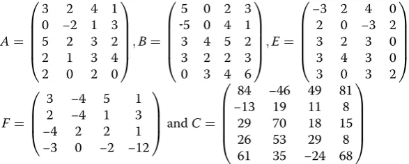
Example 4.1
A¼
3 2 4 1
0 −2 1 3
5 2 3 2
2 1 3 4
2 0 2 0
0 B B B B @
1 C C C C A;B¼
5 0 2 3
‐5 0 4 1
3 4 5 2
3 2 2 3
0 3 4 6
0 B B B B @
1 C C C C A;E¼
−3 2 4 0
2 0 −3 2
3 2 3 0
3 4 3 0
3 0 3 2
0 B B B B @
1 C C C C A
F¼
3 −4 5 1
2 −4 1 3
−4 2 2 1
−3 0 −2 −12
0 B B @
1 C C
AandC¼
84 −46 49 81
−13 19 11 8
29 70 18 15
26 53 29 8
61 35 −24 68
0 B B B B @
1 C C C C A
Choosing arbitrary initial matrices V1=W1= 0. Applying Algorithm 2.1, we get the reflexive solutions of the matrix Eq. (2.1) as follows:
V28¼
1:0000 3:0000 0:0000 0:0000
−2:0000 2:0000 0:0000 0:0000
0:0000 0:0000 2:0000 1:0000
0:0000 0:0000 4:0000 2:0000
0 B B @
1 C C
A∈R44r ð ÞP
andW28 ¼
2:0000 1:0000 0:0000 0:0000
3:0000 3:0000 0:0000 0:0000
0:0000 0:0000 4:0000 2:0000 0:0000 0:0000 −1:0000 3:0000
0 B B @
1 C C
A∈R4rx4ð ÞS
whereP¼S¼
1 0 0 0
0 1 0 0
0 0 −1 0
0 0 0 −1
0 B B @
1 C C
A, with the corresponding residual
‖R28‖=‖C−(AV28+BW28−EV28F)‖= 6.8125 × 10⁻¹⁰. Moreover, It can be verified that PV28P=V28 and SW28S=W28. Table 1 indicates the number of iterations k and norm of the corresponding residual:
Now letV^ ¼
1 1 0 0
−1 −1 0 0
0 0 −2 1
0 0 3 −1
0 B B @
1 C C A;W^ ¼
1 −1 0 0
1 −1 0 0
0 0 1 2
0 0 −2 1
0 B B @
1 C C A.
By applying Algorithm 2.1 for the generalized Sylvester matrix equation AVþBW ¼EV FþC; and letting the initial pair V1¼W1¼0, we can obtain the least Frobenius norm generalized solution V;W of the generalized Sylvester matrix Eq. (2.1) as follows
Table 1The number of iterations and norm of the corresponding residual for the reflexive solution of the generalized Sylvester matrix equation Example 4.1
Number of iterationsk Norm of the corresponding residual‖R‖
26 1.1974 × 10⁻⁸
27 6.9049 × 10⁻⁹
28 6.8125 × 10⁻¹⁰
V¼V29¼
−0:0000 2:0000 0:0000 0:0000
−1:0000 3:0000 0:0000 0:0000
0:0000 0:0000 4:0000 0:0000
0:0000 0:0000 1:0000 3:0000
0 B B @
1 C C A;
W¼W29¼
1:0000 2:0000 0:0000 0:0000 2:0000 4:0000 0:0000 0:0000 0:0000 0:0000 3:0000 −0:0000 0:0000 0:0000 1:0000 2:0000
0 B B @
1 C C
A , with the corresponding
residual
R29
k k ¼kC−ðAV29þBW29−EV29FÞk ¼ 5:089610−11:
Table 2indicates the number of iterationskand norm of the corresponding residual withV1 ¼W1¼0.
Example 4.2
(Special case) Consider the generalized Sylvester matrix equation AV+BW=EVF+C
where
A¼
−0:2 1 0 0
1 −0:1 0 0
0 0 −0:3 0
0 0 0 0:4
0 B B @
1 C C
A;E¼
2 0 0 0
0 1 0 0
0 0 3 0
0 0 0 2
0 B B @
1 C C
A;B¼
−2 1 0 0
−1 4 0 0
0 0 −3 0
0 0 0 3
0 B B @
1 C C A
F¼
2 0 0 0
0 1 0 0
0 0 −0:2 0
0 0 0 4
0 B B @
1 C C
AandC¼
1 0 0 0
0 −0:2 0 0
0 0 1 0
0 0 −0:1 3
0 B B @
1 C C A
Choosing arbitrary initial iterative matrices V1¼W1¼0. Applying Algorithm 2.1, we get the reflexive solutions of the matrix Eq.(2.1) after 7 iterations whenε= 10−10as follows:
V7¼
‐0:177130 ‐0:016697 0:000000 0:000000
0:041119 0:014553 0:000000 0:000000 0:000000 0:000000 0:033003 0:000000 0:000000 0:000000 ‐0:008300 ‐0:341520
0 B B @
1 C C
A∈R44r ð ÞP and
W7¼
‐0:085183 0:005417 0:000000 0:000000
0:044574 ‐0:040468 0:000000 0:000000
0:000000 0:000000 ‐0:330030 0:000000
0:000000 0:000000 ‐0:031125 0:134810
0 B B @
1 C C
A∈R44r ð ÞS
Table 2The number of iterations and norm of the corresponding residual for Example 4.1 withV1
¼W1¼0
Number of iterationsk Norm of the corresponding residual‖R‖
26 2.9491×10‐7
27 6.3498×10‐7
28 2.5150×10‐9
29 5.0896×10‐11
whereP¼
1 0 0 0
0 1 0 0
0 0 −1 0
0 0 0 −1
0 B B @ 1 C C
AandS=P.
It can be verified that PV7P=V7 and SW7S=W7. Moreover, the corresponding re-sidual‖R7‖=‖C−AV7+EV7F−BW7‖= 8.1907e−10.
Example 4.3
Consider the generalized Sylvester matrix equationAV+BW=EVF+Cwhere
A¼
2 ‐1 ‐3 3 ‐1 0 3 ‐1 1 ‐2 0 2 3 2 0 1 4 ‐3 2 ‐1 3 2 0 ‐3 4 ‐1 2 ‐2 3 1 2 ‐1 0 3 ‐2 1
0 B B B B B B @ 1 C C C C C C A
;E¼
4 ‐3 1 2 0 ‐2 0 2 4 1 ‐2 3
‐2 0 4 3 2 ‐3 1 ‐2 4 2 0 3 3 ‐2 1 4 1 2 1 2 0 ‐2 ‐3 4
0 B B B B B B @ 1 C C C C C C A
;B¼
1 0 ‐2 ‐1 3 4 2 ‐3 3 4 0 2 1 0 3 ‐2 2 ‐3 2 ‐1 4 0 ‐3 1 0 ‐1 0 2 3 1 2 ‐1 3 ‐3 4 1
0 B B B B B B @ 1 C C C C C C A F¼
3 2 0 ‐1 ‐2 1 1 ‐1 4 2 1 ‐3
‐3 2 ‐1 0 2 1 0 ‐1 2 ‐3 1 4 2 ‐1 4 0 2 3 2 ‐1 3 2 ‐3 1
0 B B B B B B @ 1 C C C C C C A
andC¼
0 ‐11 1 22 ‐30 14
‐37 19 ‐122 ‐22 ‐4 28 65 ‐21 4 32 ‐77 ‐9 12 7 ‐77 5 ‐36 ‐65
‐11 33 ‐67 60 ‐52 ‐43
‐37 19 ‐68 ‐39 61 3
0 B B B B B B @ 1 C C C C C C A
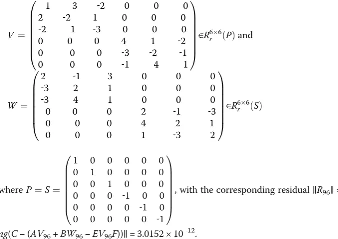
Choosing arbitrary initial matricesV1¼W1¼0. Applying Algorithm 2.1, we get the reflexive solutions of the matrix Eq. (2.1) after108iterations whenε= 10−10as follows:
V ¼
1 3 ‐2 0 0 0
1 3 ‐2 0 0 0
1 3 2 0 0 0
0 0 0 2 1 ‐2
0 0 0 2 1 ‐2
0 0 0 2 1 2
0 B B B B B B @ 1 C C C C C C A
∈R66r ð ÞP and
W ¼
2 ‐1 3 0 0 0
2 ‐1 3 0 0 0
2 ‐1 ‐3 0 0 0
0 0 0 2 ‐1 3
0 0 0 2 ‐1 3
0 0 0 2 ‐1 ‐3
0 B B B B B B @ 1 C C C C C C A
∈R66r ð ÞS
whereP¼S¼
1 0 0 0 0 0
0 1 0 0 0 0
0 0 1 0 0 0
0 0 0 ‐1 0 0
0 0 0 0 ‐1 0
0 0 0 0 0 ‐1
0 B B B B B B @ 1 C C C C C C A
, with the corresponding residual
‖R108‖=‖C−(AV108+BW108−EV108F)‖= 3.0452 × 10⁻¹⁰. Moreover, It can be verified thatPV108P=V108andSW108S=W108. Table3indicates the number of iterationskand norm of the corresponding residual:
Example 4.4
A¼
2 ‐1 ‐3 3 ‐1 0 5 ‐2 0 5 1 ‐3 3 ‐1 1 ‐2 0 6 1 5 ‐3 ‐2 0 3 3 2 0 ‐5 4 ‐3 2 ‐1 3 ‐5 0 ‐3 4 ‐1 2 ‐2 3 1 2 ‐1 0 3 ‐2 1
0 B B B B B B B B B B @ 1 C C C C C C C C C C A
;E¼
4 ‐3 1 2 0 ‐2
0 2 4 1 ‐2 3
‐2 0 4 3 2 ‐3
3 ‐2 5 4 3 0
1 ‐2 4 2 0 3
1 ‐3 2 4 0 2
3 ‐2 1 4 1 2
‐1 2 0 ‐2 ‐3 4
0 B B B B B B B B B B @ 1 C C C C C C C C C C A B¼
1 0 ‐2 ‐1 3 4 3 ‐5 ‐3 2 4 1
2 ‐3 3 4 0 2
1 0 3 ‐2 2 ‐3
‐4 5 ‐3 4 ‐1 0
2 ‐1 4 0 ‐3 1
0 ‐1 0 2 3 1
2 ‐1 3 ‐3 4 1
0 B B B B B B B B B B @ 1 C C C C C C C C C C A ; F¼
3 2 0 ‐1 ‐2 1 1 ‐1 4 2 1 ‐3
‐3 2 ‐1 0 2 1
0 ‐1 2 ‐3 1 4
2 ‐1 4 0 2 3
2 ‐1 3 2 ‐3 1
0 B B B B B B @ 1 C C C C C C A
andC¼
‐11 ‐51 ‐58 29 ‐15 68
‐27 85 ‐124 52 ‐26 ‐82 59 ‐93 109 39 ‐6 28
‐18 22 ‐24 ‐14 ‐5 86
‐59 125 ‐144 ‐41 ‐68 ‐11
‐40 56 ‐105 ‐5 ‐89 ‐27
‐43 43 ‐110 15 ‐53 ‐10
‐54 144 ‐109 14 20 ‐75
0 B B B B B B B B B B @ 1 C C C C C C C C C C A
Choosing arbitrary initial matricesV1¼W1¼0. Applying Algorithm 2.1, we get the reflexive solutions of the matrix Eq. (2.1) after96iterations whenε= 10−12as follows:
V ¼
1 3 ‐2 0 0 0
2 ‐2 1 0 0 0
‐2 1 ‐3 0 0 0
0 0 0 4 1 ‐2
0 0 0 ‐3 ‐2 ‐1
0 0 0 ‐1 4 1
0 B B B B B B @ 1 C C C C C C A
∈R66r ð ÞP and
W ¼
2 ‐1 3 0 0 0
‐3 2 1 0 0 0
‐3 4 1 0 0 0
0 0 0 2 ‐1 ‐3
0 0 0 4 2 1
0 0 0 1 ‐3 2
0 B B B B B B @ 1 C C C C C C A
∈R66r ð ÞS
whereP¼S¼
1 0 0 0 0 0
0 1 0 0 0 0
0 0 1 0 0 0
0 0 0 ‐1 0 0
0 0 0 0 ‐1 0
0 0 0 0 0 ‐1
0 B B B B B B @ 1 C C C C C C A
, with the corresponding residual‖R96‖=‖
diag(C−(AV96+BW96−EV96F))‖= 3.0152 × 10⁻¹².
Table 3The number of iterations and norm of the corresponding residual for the reflexive solution of the generalized Sylvester matrix equation Example 4.3
Number of iterationsk Norm of the corresponding residual‖R‖
89 7.3204×10‐8
99 5.5252×10‐9
108 3.0452×10‐10
127 2.6502×10‐12
Table 4The number of iterations and norm of the corresponding residual for the reflexive solution of the generalized Sylvester matrix equation Example 4.4
Number of iterationsk Norm of the corresponding residual‖R‖
77 1.2455×10‐6
81 2.1035×10‐8
84 2.2031×10‐10
Moreover, It can be verified thatPV96P=V96andSW96S=W96. Table4indicates the number of iterationskand norm of the corresponding residual.
Conclusions
In this paper, an iterative method to solve the generalized Sylvester matrix equa-tions over reflexive matrices is derived. With this iterative method, the solvability of the generalized Sylvester matrix equation can be determined automatically. Also, when this matrix equation is consistent, for any initial reflexive matrices, one can obtain reflexive solutions within finite iteration steps. In addition, both the com-plexity and the convergence analysis for our proposed algorithm are presented. Furthermore, we obtained the least Frobenius norm reflexive solutions when special initial reflexive matrices are chosen. Finally, four numerical examples were pre-sented to support the theoretical results and illustrate the effectiveness of the pro-posed method.
Acknowledgements
The authors are grateful to the referees for their valuable suggestions.
Authors’contributions
MAR proposed the main idea of this paper. MAR and NME-S prepared the manuscript and performed all the steps of the proofs in this research. BIS has made substantial contributions to conception and designed the numerical methods. All authors contributed equally and significantly in writing this paper. All authors read and approved the final manuscript.
Authors’information
Mohamed A. Ramadan works in Egypt as Professor of Pure Mathematics (Numerical Analysis) at the Department of Mathematics and Computer Science, Faculty of Science, Menoufia University, Shebein El-Koom, Egypt. His areas of ex-pertise and interest are: eigenvalue assignment problems, solution of matrix equations, focusing on investigating, the-oretically and numerically, the positive definite solution for class of nonlinear matrix equations, introducing numerical techniques for solving different classes of partial, ordering and delay differential equations, as well as fractional differ-ential equations using different types of spline functions. Naglaa M. El-Shazly works in Egypt as Assistant Professor of Pure Mathematics (Numerical Analysis) at the Department of Mathematics and Computer Science, Faculty of Science, Menoufia University, Shebein El-Koom, Egypt. Her areas of expertise and interest are: eigenvalue assignment problems, solution of matrix equations, theoretically and numerically, iterative positive definite solutions of different forms of nonlinear matrix equations. Basem I. Selim works in Egypt as Assistant Lecturer of Pure Mathematics at the Department of Mathematics and Computer Science, Faculty of Science, Menoufia University, Shebein El-Koom, Egypt. His research interests include Finite Element Analysis, Numerical Analysis, Differential Equations and Engineering, Applied and Com-putational Mathematics.
Funding
Not applicable.
Availability of data and materials
All data generated or analyzed during this study are included in this article.
Competing interests
The authors declare that they have no competing interests.
Received: 9 March 2019 Accepted: 17 July 2019
References
1. Horn, R.A., Johnson, C.R.: Topics in matrix analysis. Cambridge University Press, England (1991)
2. Golub, G.H., Van Loan, C.F.: Matrix computations, 3rd edn. The Johns Hopkins University Press, Baltimore and
London (1996)
3. Chen, H.C.: Generalized reflexive matrices: special properties and applications. SIAM J. Matrix Anal. Appl.19,
140–153 (1998)
4. Peng, X.Y., Hu, X.Y., Zhang, L.: An iteration method for the symmetric solutions and the optimal approximation solution of the matrix equationAXB=C. Appl. Math. Comput.160, 763–777 (2005)
5. Peng, X.Y., Hu, X.Y., Zhang, L.: The reflexive and anti-reflexive solutions of the matrix equationAHXB=C. Appl. Math. Comput.186, 638–645 (2007)
7. Zhan, J.C., Zhou, S.Z., Hu, X.Y.: The (P,Q) generalized reflexive and anti-reflexive solutions of the matrix equationAX=B. Appl. Math. Comput.209, 254–258 (2009)
8. Ramadan, M.A., Abdel Naby, M.A., Bayoumi, A.M.: On the explicit and iterative solutions of the matrix equation
AV+BW=EVF+C. Math. Comput. Model.50, 1400–1408 (2009)
9. Dehghan, M., Hajarian, M.: An iterative algorithm for the reflexive solutions of the generalized coupled Sylvester matrix equations and its optimal approximation. Appl. Math. Comput.202, 571–588 (2008)
10. Dehghan, M., Hajarian, M.: Finite iterative algorithms for the reflexive and anti-reflexive solutions of the matrix equation
A1X1B1+A2X2B2=C. Math. Comput. Model.49, 1937–1959 (2009)
11. Yin, F., Guo, K., Huang, G.X.: An iterative algorithm for the generalized reflexive solutions of the general coupled matrix equations. Journal of Inequalities and Applications.2013, 280 (2013)
12. Li, N.: Iterative algorithm for the generalized (P, Q) - reflexive solution of a quaternion matrix equation with j-conjugate of the unknowns. Bulletin of the Iranian Mathematical Society.41, 1–22 (2015)
13. Dong, C.Z., Wang, Q.W.: The {P,Q,k+l}- reflexive solution to system of matricesAX=C,XB=D. Mathematical Problems in Engineering.2015, 9 (2015)
14. Nacevska, B.: Generalized reflexive and anti-reflexive solution for a system of equations. Filomat.30, 55–64 (2016) 15. Hajarian, M.: Convergence properties of BCR method for generalized Sylvester matrix equation over generalized reflexive
and anti-reflexive matrices. Linear and Multilinear Algebra.66(10), 1–16 (2018)
16. Liu, X.: Hermitian and non-negative definite reflexive and anti-reflexive solutions toAX=B. International Journal of Computer Mathematics.95(8), 1666–1671 (2018)
17. Dehghan, M., Shirilord, A.: A generalized modified Hermitian and skew–Hermitian splitting (GMHSS) method for solving complex Sylvester matrix equation. Applied Mathematics and Computation.348, 632–651 (2019)
18. Dehghan, M., Hajarian, M.: On the reflexive and anti–reflexive solutions of the generalized coupled Sylvester matrix equations. International Journal of Systems Science.41(6), 607–625 (2010)
19. Dehghan, M., Hajarian, M.: On the generalized bisymmetric and skew–symmetric solutions of the system of generalized Sylvester matrix equations. Linear and Multilinear Algebra.59(11), 1281–1309 (2011)
20. Hajarian, M., Dehghan, M.: The reflexive and Hermitian reflexive solutions of the generalized Sylvester–conjugate matrix equation. The Bulletin of the Belgian Mathematical Society.20(4), 639–653 (2013)
21. Dehghan, M., Hajarian, M.: Two algorithms for finding the Hermitian reflexive and skew–Hermitian solutions of Sylvester matrix equations. Applied Mathematics Letters.24(4), 444–449 (2011)
22. Hajarian, M.: Solving the coupled Sylvester like matrix equations via a new finite iterative algorithm. Engineering Computations.34(5), 1446–1467 (2017)
23. El-Shazly, N.M.: On the perturbation estimates of the maximal solution for the matrix equationXþATpffiffiffiffiffiffiffiX−1A¼P.
Journal of the Egyptian Mathematical Society.24, 644–649 (2016)
24. Khader, M.M.: Numerical treatment for solving fractional Riccati differential equation. Journal of the Egyptian Mathematical Society.21, 32–37 (2013)
25. Balaji, S.: Legendre wavelet operational matrix method for solution of fractional order Riccati differential equation. Journal of the Egyptian Mathematical Society.23, 263–270 (2015)
26. Moore, B.: Principle component analysis in linear systems: controllability, observability and model reduction. IEEE Transactiona on Automatic Control.26, 17–31 (1981)
27. Kenney, C.S., Laub, A.J.: Controllability and stability radii for Companion form systems. Mathematics Control Signals and Systems.1, 239–256 (1988)
28. Lam, J., Yan, W., Hu, T.: Pole assignment with eigenvalue and stability robustness. International Journal of Control.
72, 1165–1174 (1999)
29. Avrachenkov, K.E., Lasserre, J.B.: Analytic perturbation of Sylvester matrix equation. IEEE Transactiona on Automatic Control.47, 1116–1119 (2002)
Publisher’s Note