www.adv-radio-sci.net/5/209/2007/ © Author(s) 2007. This work is licensed under a Creative Commons License.
Radio Science
Adaptive decoding of convolutional codes
K. Hueske, J. Geldmacher, and J. G¨otze
Information Processing Lab - AG DT, University of Dortmund, Germany
Abstract. Convolutional codes, which are frequently used as error correction codes in digital transmission systems, are generally decoded using the Viterbi Decoder. On the one hand the Viterbi Decoder is an optimum maximum likelihood decoder, i.e. the most probable transmitted code sequence is obtained. On the other hand the mathematical complexity of the algorithm only depends on the used code, not on the number of transmission errors. To reduce the complexity of the decoding process for good transmission conditions, an alternative syndrome based decoder is presented. The reduc-tion of complexity is realized by two different approaches, the syndrome zero sequence deactivation and the path metric equalization. The two approaches enable an easy adaptation of the decoding complexity for different transmission con-ditions, which results in a trade-off between decoding com-plexity and error correction performance.
1 Introduction
The Viterbi Decoder (VD) (Viterbi, 1967) is the standard ap-proach for decoding convolutional codes. The decoder is based on the application of the Viterbi Algorithm (VA) to the trellis representation of the convolutional encoder. For-ney Jr. (1973) furthermore showed that the Viterbi Decoder is an optimum Maximum Likelihood (ML) decoder, i.e. the valid code sequence with minimum distance to the received sequence is obtained.
The mathematical complexity only depends on the used code, i.e. it is not depending on the channel behaviour, which will be described as Signal to Noise Ratio (SNR) in this pa-per. This means, a constant high amount of decoding opera-tions is required, even if few or no errors occurred. This is a
Correspondence to: K. Hueske
disadvantage, especially for applications that require energy efficient implementations (e.g. mobile terminals).
This paper presents an alternative syndrome based con-volutional decoder, whose complexity can be adaptively re-duced in case of good transmission conditions. The decoder also uses the VA, but the algorithm is applied to the trellis representation of the syndrome former. While the VD deter-mines the most likely transmitted code sequence directly, the syndrome based decoder determines the most probable error sequence first. It will be shown that both methods allow op-timum ML decoding, but using the syndrome former trellis is advantegous in terms of adaptivity and complexity.
Syndrome based convolutional decoders were also de-scribed by Schalkwijk and Vinck (1975); Ariel and Snyders (1999); Reed and Truong (1985), but the presented decoder allows further adaptivity in terms of a trade-off between com-putational complexity and error correction performance. The reduction in complexity is realized using two approaches: The syndrome zero sequence deactivation considers the de-pendencies between the syndrome and the error sequence, which allows the deactivation of the decoder for error free sequences. This leads to a reduction of decoding complexity for high SNR with no or marginal loss in decoding perfor-mance.
The path metric equalization reduces the required number of Add-Compare-Select (ACS) operations for the VA by us-ing identical path metrics for different error patterns. The error correction performance is decreased but the decoding complexity can be reduced by 25%. This is especially useful for applications that require a BER threshold and do not ben-efit from further BER degradation. While the performance of the presented decoder without adaptation is equivalent to the standard VD, we can reduce the complexity of the decoding process if the BER is below the required threshold.
that both are optimum ML decoders. In Sect. 3 two meth-ods for complexity reduction are introduced, syndrome zero sequence deactivation and path metric equalization. Further-more an estimation technique for the Bit Error Rate (BER) is introduced, which is used for an adaptive complexity reduc-tion. For performance and complexity analysis simulation results are presented in Sect. 4. Conclusions are given in Sect. 5.
2 Syndrome decoding
In this section the syndrome decoding algorithm proposed by Schalkwijk and Vinck (1975) is presented.
2.1 Syndrome decoding
The syndrome decoding algorithm is presented for code rates R=k/n. Sequences and transfer functions are represented in frequency domain as power series inDwith coefficients fromGF (2). For the sake of clarity, the delay operatorDis omitted in the following.
An information sequence is encoded by multiplication with a generator matrix
v=uG, (1)
where G is a polynomial generator matrix withkrows andn columns, v is a row vector of lengthncontaining the coded bits and u is a row vector of lengthkcontaining the informa-tion bits.
The sequence v is transmitted over a memoryless, noisy channel, causing the corrupted received sequence
r=v+e, (2)
where e is the error sequence resulting from channel noise. A syndrome sequence b is computed from the received sequence as
b=rHT, (3)
where HT is a polynomial matrix withn rows and n−k columns and is called the syndrome former matrix of G. The syndrome former matrix is defined to be orthogonal to G, thus the syndrome sequence b is the zero sequence if and only if r is a valid code sequence. It follows that the syn-drome sequence only depends on the error sequence and is independent of the transmitted information:
b=rHT =(v+e)HT =eHT (4)
The syndrome decoder has to map the syndrome sequence back to the error sequence. However the mapping from b to e is not unique, but there is a set of error sequences correspond-ing to one syndrome sequence. For ML decodcorrespond-ing the decoder has to determine the code sequence with minimum distance to the received sequence, which corresponds to the error se-quence with minimum weight. Thus the decoding problem
can be formulated in terms of an optimization problem with constraint:
min
ˆ
e
||ˆe|| with b= ˆeHT (5) The norm||...||is defined as hamming distance for hard de-cision decoding and as 2-norm for soft dede-cision decoding. The minimization can be done by searching the syndrome former trellis for the error sequence with minimum weight using the VA. The constraint is incorporated by only allow-ing the transitions belongallow-ing to the current syndrome value at every stage in the syndrome former trellis.
When the ML error sequencee has been found, the trans-ˆ mission errors are corrected by subtracting the estimated er-ror sequence from the received sequence
ˆ
v=r− ˆe, (6)
wherev is the estimated code sequence. Finally the informa-ˆ tion sequence can be obtained as the product of the estimated code sequence and the right inverse generator matrix
ˆ
u= ˆvG−1. (7)
2.2 Syndrome former matrix and trellis representation The syndrome former HT can be calculated from the invari-ant factor decomposition (IFD) of the generator matrix G. The IFD of a matrix G is defined as
G=A0B (8)
where A is a polynomial (k×k) matrix and B is a polynomial (n×n) matrix with det(A)=det(B)=1. 0is a (k×n) matrix and is called Smith-Form of G. An algorithm for the compu-tation and the properties of the IFD are given in Johannesson and Zigangirov (1999).
The firstkrows of B form an equivalent generator matrix of G and the lastn−krows are the transpose of the inverse of H:
B=
Gb
(H−1)T
(9) As B is non-singular, it can be inverted. The right inverse equivalent generator matrix G−b1 and the syndrome former HT can be identified as the firstkcolumns and the lastn−k
columns of B−1, respectively:
B−1= G−b1HT (10)
7 6 5 4 3 2 1 0
Switch Decoder Off
Switch Decoder On
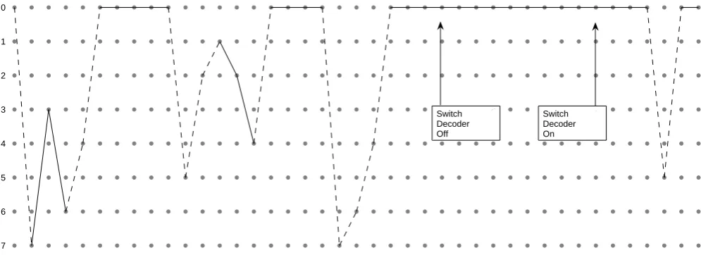
Fig. 1. Example of an error path, “0“-syndrome sequences are plotted as lines, ”1“-syndrome sequences are plotted dashed.
2vstates, wherevis the number of memory elements of the encoder, and 2nedges leaving each state.
ForR=1/2 the syndrome trellis has 4 edges leaving each state. The trellis can be split into two parts, with each part containing only the transitions of one syndrome sym-bol. This results in two trellises with each 2v states and 2 edges leaving each state.
To find the minimum weight error sequence, a shortest path algorithm like the VA is used. As branch metric for the transition of a state to a successor state, the weight of the corresponding error pattern is taken. To incorporate the con-straint from Eq. (5), at each decoding stage only the trellis part corresponding to the current syndrome symbol is con-sidered.
2.3 Equivalence to the Viterbi Decoder
The equivalence of the syndrome based decoder to the VD can be shown by replacing the estimated errore in Eq. (5) byˆ r− ˆv. Expression (5) then becomes
min
ˆ
v
||r− ˆv||with b=(vˆ+ ˆe)HT, (11)
and using b= ˆeHT leads to min
ˆ
v
||r− ˆv||with 0= ˆvHT, (12) which represents the decoding problem in “Viterbi sense“. As both decoders are equivalent, the syndrome based decoder is also an optimum ML decoder.
We note that the syndrome computation in Eq. (3) and the mapping from estimated code sequence to information se-quence in Eq. (7) can be realized as simple XOR operations. Thus the estimation of the error sequence has a similar com-plexity as the VD.
3 Adaptive decoding
3.1 Syndrome zero sequence deactivation
Good transmission conditions will lead to error free se-quences in r, i.e. to sese-quences where e=0. As the syndrome sequence only depends on the channel errors, as shown in Eq. (4), error free periods will lead to zero sequences in the syndrome b, too. For zero sequences, no decoding is neces-sary, the zero path in the syndrome former trellis is taken.
The first proposed optimization of the syndrome decoder now consists of detecting zero sequences in the syndrome, and switching the decoder off for these sequences. A reason-able length of the period has to be assumed, to be sure, that the ML path in the trellis has returned to zero state. Decoding is done by always tracing back from zero state.
If the minimum zero period length is chosen long enough, the decoding performance can be as good as the performance of the unmodified decoder. There is a trade-off, decoding performance can be exchanged with decoding complexity by reducing or increasing the required length of the zero se-quences.
There are two critical parameters for the adaptive decoder: The first parameterloffis the number of syndrome zeros,
af-ter which the decoder can be safely switched off. The second parameterlon is the number of stages before the first
7
00
11
6
00 11
5
00
11 4
00 11 3
01
10 2
01 10
1 01
10 0
01 10
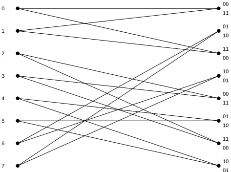
Fig. 2. Syndrome former trellis for the example code, Syndrome 0
part.
As an example, Fig. 1 shows an error path for av=3 Code. In this example the decoder is switched off, when six suc-cessive syndrome zeros are detected. The decoder is turned off afterloff=3 syndrome zeros and turned on againlon=3
stages before the next syndrome one.
3.2 Path metric equalization
A second reduction of the computational complexity is based on a closer examination of the syndrome former trellis struc-ture. As Schalkwijk et al pointed out in Schalkwijk and Vinck (1976), the syndrome former trellis has a special struc-ture. We can identify pairs of states which have the same pre-decessor states and at the same time have identical weights of the corresponding transition in case of hard decision.
For example, Fig. 2 shows a syndrome former trellis for a code with memory length v=3 and generator polynomials G=[D3+D2+1, D3+D2+D+1]. For simplicity only the zero part is considered. The trellis is annotated on the left side with the state numbers and on the right side with the er-ror input corresponding to the transition. One can see that the states 1 and 3 have the same predecessor states (6 and 7) with the transitions having the same weight 0+1=1 and 1+0=1. The same holds for the states 5 and 7 which have the predecessors 4 and 5.
LetM(i)(t )be the metric of stateiat timet andµ(i,j )(t ) the branch metric for a transition from stateito statej. At every decoding stage and for every state the VA has to com-pute the metrics for all transitions from each predecessor state, compare the metrics and choose the survivor path as the path with minimum metric (ACS). For example, for the
states 1 and 3 the metric is computed as M(1)(t+1)=
min{M(6)(t ) +µ(6,1)(t ), M(7)(t )+µ(7,1)(t )} M(3)(t+1)=
min{M(6)(t ) +µ(6,3)(t ), M(7)(t )+µ(7,3)(t )}
(13)
If harddecision is applied, the branch metrics are com-puted as
µ(6,1)(t )=µ(7,3)(t )=0+1=1
µ(7,1)(t )=µ(6,3)(t )=1+0=1 (14) and Eq. (13) becomes
M(1)(t+1)=min{M(6)(t )+1, M(7)(t )+1}
M(3)(t+1)=min{M(6)(t )+1, M(7)(t )+1} (15) The metric computation is identical for both state 1 and state 3 and thus for state 3 no computation is required. The same holds for states 6 and 7.
We can use this for reducing the complexity of the decoder and save one ACS operation for each of the 2v−2pairs. If the decoder uses harddecision, 25% of the ACS operations can be saved without loss of decoding performance (Schalkwijk and Vinck, 1976).
However as hard decision is rarely used, we now dis-cuss the metric computation for the soft decision case. Let r(t )=[r1(t ) r2(t )]be the 3-Bit quantized vector received at
timet, zero symmetric BPSK modulation and AWGN chan-nel assumed. The absolute value of r(t )can be seen as a mea-sure for the confidence of the received word. The lower the absolute value ofri(t ), the more likely a transmission error
occurred at this position. Thus the branch metric calculation for softdecision can formulated as
<e(t ),r(t ) >= [e1(t ) e2(t )][|r1(t )| |r2(t )|]T (16)
to incorporate the confidence informations. The metric cal-culation for the example becomes
M(1)(t+1)=min{M(6)(t )+ |r2(t )|, M(7)(t )+ |r1(t )|}
M(3)(t+1)=min{M(6)(t )+ |r1(t )|, M(7)(t )+ |r2(t )|}
(17) So the metric calculation is not identical for soft decision and a simplification is no longer possible without decoding performance loss.
However, the metric calculation can be modified to allow a simplification analog to the hard decision case. This is re-alized by assigning the same branch metrics to the 01 and 10 error patterns, which can be done by choosing the mini-mum of|r1(t )|and|r2(t )|as branch metric for the 01 and 10
transitions:
µ(i,j )(t )=
0 for e(t )= [00]
min{|r1(t )|,|r2(t )|} for e(t )= [10]
min{|r1(t )|,|r2(t )|} for e(t )= [01]
0 1 2 3 4 5 6 7 8 9 10 0
5 10 15 20 25 30 35 40 45 50
Eb/N0 [dB]
Percentage non−zero elements [%]
Non−zero elements in syndrome sequence
Fig. 3. Percentage of non-zero elements in syndrome vector.
The metric computation for the states 3 and 6 then becomes M(1)(t+1)=min{M(6)(t )+min{|r1(t )|,|r2(t )|},
M(7)(t )+min{|r1(t )|,|r2(t )|}}
M(3)(t+1)=min{M(6)(t )+min{|r1(t )|,|r2(t )|},
M(7)(t )+min{|r1(t )|,|r2(t )|}} (18)
If the metric calculation is modified in this way, the reduction of complexity can be applied as in the hard decision case. However, there will be a loss of decoding performance com-pared to the full complexity soft decision decoder.
3.3 BER estimation
The path metric equalization is especially suitable for trans-mission systems that require a specific BER and do not benefit from better channel conditions. If the desired BER is reached, the complexity of the decoder can be reduced adaptively. The total error correction performance will be decreased, but the required BER threshold will always be achieved.
The problem that comes up with this approach is that the BER is generally unknown in the receiver. But using the syn-drome vector we can roughly estimate the BER by calculat-ing the syndrome vector weight. This means for good trans-mission conditions only few errors occur, which results in a syndrome vector with only few non-zero elements. On the other hand if the SNR is very low, we expect many transmis-sion errors, which produces many non-zero elements. The dependencies between SNR and number of non-zero ele-ments in the syndrome vector is depicted in Fig. 3.
Using this relation we can define a syndrome vector weight threshold in the receiver, which allows an adaptive switching between the normal and the reduced complexity syndrome based decoder.
1 1.5 2 2.5 3 3.5 4 4.5 5 5.5 10−5
10−4 10−3 10−2 10−1
100
E
b/N0 [dB]
BER
Uncoded
Simplified syndrome decoder Adaptive syndrome decoder Syndrome decoder
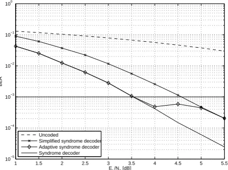
Fig. 4. Comparison of the Bit-Error-Rates of the reduced
complex-ity decoder and the full complexcomplex-ity decoder.
3.4 Summary
There are two options for reduction of decoding complexity. The first option is an adaptive decoding approach, which is based on analyzing the syndrome sequence and turning off the decoder in error-free periods. A reasonable minimum length assumed, decoding costs can be reduced without loos-ing decodloos-ing performance. The second option is based on the syndrome former trellis structure and allows a reduction of decoding complexity by about 25% but resulting in a loss of decoding performance.
4 Simulation results
This section gives simulation results for both options. All simulations have been done for a code with generator matrix G= [D3+D2+1, D3+D2+D+1] (19) withv=3 path registers and corresponding syndrome former HT = [D3+D2+D+1, D3+D2+1]T (20) The codewords are transmitted over a memoryless AWGN channel using BPSK modulation. For the BER simulations soft decision was applied, considering 2000 simulated errors. Figure 4 shows the results for the reduced complexity syn-drome decoder using path metric equalization. The per-formance of the simplified syndrome decoder is about 1dB worse compared to the regular syndrome decoder, but it re-quires 25% less operations. The same figure shows the adap-tive decoding approach with a desired BER of 10−3. For a Eb/N0< 3.5 dB only the unmodified syndrome decoder is
1 1.5 2 2.5 3 3.5 4 4.5 5 5.5 10−5
10−4 10−3 10−2 10−1 100
Eb/N0 [dB]
BER
Uncoded 1 starting zero 3 starting zeros 5 starting zeros Regular Softdecision
Fig. 5. Comparison of the Bit-Error-Rates of the adaptive decoders
using 3 different minimum zero sequence lengths and the regular decoder for Softdecision.
data block. ForEb/N0>5.0 dB all decoding operations are
done by the reduced complexity decoder. This shows, that the decoding complexity can be easily adapted for different channel conditions.
Figure 5 shows the performance of the decoder using syn-drome zero sequence deactivation. Simulations are shown forlon=3 andloff ∈ {1,3,5}. In Fig. 6 the percentage of the
decoding time the decoder is turned off is plotted. For ex-ample atEb/N0=4.5 dB the decoder withloff=5 is turned
off about 33% of the time with about 0.15 dB loss in perfor-mance compared to the regular decoder. This allows a reduc-tion of complexity with only marginal performance loss. If desired, the complexity can be further decreased by reducing loff. AtEb/N0=4.5 dB the decoder withloff=1 is turned
off about 48% of the time while taking a loss of about 1 dB.
5 Conclusions
While performance and computational complexity of the Syndrome Decoder are equivalent to the Viterbi Decoder for worst case transmission conditions, the syndrome based de-coder allows an adaptive reduction of complexity for good channel conditions. With the proposed methods the adaptive reduction can be performed in two steps. First, the syndrome zero sequence deactivation will reduce the decoding com-plexity without significant loss in decoding performance. If desired, the required number of operations can be further de-creased by either using a reduced lengthloff or using the
path metric equalization. The last step is especially appli-cable for transmission systems that require a BER threshold and do not benefit from further SNR improvement.
1 1.5 2 2.5 3 3.5 4 4.5 5 5.5 0
10 20 30 40 50 60 70
Eb/N0 [dB]
Turned off decoder [%]
1 starting zero 3 starting zeros 5 starting zeros
Fig. 6. The percentage of turned off decoders for th 3 different
minimum zero sequence lengths.
References
Ariel, M. and Snyders, J.: Error-trellises for convolutional codes .II. Decoding methods, Communications, IEEE Transactions on, 47, 1015–1024, doi:10.1109/26.774852, 1999.
Forney Jr., G.: Convolutional codes I: Algebraic structure, Informa-tion Theory, IEEE TransacInforma-tions on, 16, 720–738, 1970. Forney Jr., G.: The Viterbi Algorithm, IEEE Proceedings, 61, 268–
278, 1973.
Johannesson, R. and Zigangirov, K. S.: Fundamentals of Convolu-tional Coding, IEEE press, 1999.
Reed, I. and Truong, T.: Error-trellis syndrome decoding tech-niques for convolutional codes, IEE Proceedings Pt. F, 132, 77– 83, 1985.
Schalkwijk, J. and Vinck, A.: Syndrome Decoding of Convolutional Codes, Communications, IEEE Transactions on, 23, 789–792, 1975.
Schalkwijk, J. and Vinck, A.: Syndrome Decoding of Binary Rate-1/2 Convolutional Codes, Communications, IEEE Transactions on, 24, 977–985, 1976.