Adversarial Unsupervised Representation Learning for Activity Time-Series

(1)

The Thirty-Third AAAI Conference on Artificial Intelligence (AAAI-19)

Adversarial Unsupervised Representation Learning for Activity Time-Series

Karan Aggarwal,

1

Shafiq Joty,

2

Luis Fernandez-Luque,

3

Jaideep Srivastava

1

1_{University of Minnesota,}2_{Nanyang Technological University,}3_{Qatar Computing Research Institute}

[email protected], [email protected], [email protected], [email protected]

Abstract

Sufficient physical activity and restful sleep play a major role in the prevention and cure of many chronic conditions. Being able to proactively screen and monitor such chronic conditions would be a big step forward for overall health. The rapid increase in the popularity of wearable devices pro-vides a significant new source, making it possible to track the user’s lifestyle real-time. In this paper, we propose a novel unsupervised representation learning technique called activ-ity2vecthat learns and “summarizes” the discrete-valued ac-tivity time-series. It learns the representations with three com-ponents: (i) the co-occurrence and magnitude of the activ-ity levels in a time-segment, (ii) neighboring context of the time-segment, and (iii) promoting subject-invariance with ad-versarial training. We evaluate our method on four disorder prediction tasks using linear classifiers. Empirical evaluation demonstrates that our proposed method scales and performs better than many strong baselines. The adversarial regime helps improve the generalizability of our representations by promoting subject invariant features. We also show that using the representations at the level of a day works the best since human activity is structured in terms of daily routines.

Introduction

Physical activity and sleep are crucial to health and well-being. Requisite activity and sufficient sleep prevent vari-ous illnesses such as diabetes (Warburton, Nicol, and Bredin 2006). Rise in chronic conditions, mainly due to aging and unhealthy lifestyles, is putting our healthcare system under stress. The current disorder screening approach requires sub-jects to undergo various diagnosis steps, involving question-naires andpolysomnography(PSG). With increasing popu-larity of wearable devices likeFitbit, which collect detailed data about the body’s movements, there is an increased in-terest in using actigraphy for detecting sleep-related disor-ders and tracking longitudinal changes in the subject’s con-dition. Although much lower fidelity than clinical devices, availability of wearables provides a novel opportunity, ow-ing to its non-intrusive and real-time capabilities; specifi-cally, if we can develop techniques to extract information from the vast amounts of body-monitoring data. Such tech-niques could be useful to assist healthcare professionals as well as help monitor behavioral therapy, e.g., exercise.

Only a minuscule proportion of the population has both their clinical data and wearables data available. Thus a purely su-pervised approach utilizing the wearables-clinical data cor-pus is sub-optimal since it renders the activity data from a majority of subjects redundant. Hence, any approach to-wards using activity signals should utilize the unsupervised learning. Second, an important aspect is that information in actigraphy signals depends on the subjects and their envi-ronments, such as their routines and surroundings (Storm, Heller, and Mazz`a 2015) along with measurement errors ow-ing to device design. We propose a two-pronged approach. First, a mapping of the temporal relations of the activities from the time-series to a feature space should be learned. Second, this feature space should take into account the sub-ject’s environment, and make the representations invariant to the subject and their environment.

We propose a new method that addresses these challenges. Our activity2vecmethod is an unsupervised representation learning model that learns distributed representations for activity signals spanning over a time segment (e.g., at a day level) in a subject invariant manner. We use two public data-sets to evaluate our approach against baselines on four disorder prediction tasks. Using a linear classifier (logistic regression), we show our proposed representation learning method outperforms the baseline time-series methods, with day-level representations performing the best. The linear classifier with our learned features performs at par with the convolution neural network baseline trained end-to-end on the tasks. We also demonstrate the effectiveness of inducing subject invariant features.

Unlike traditional time-series methods, our feature vec-tors can be used to boost the performance of the supervised learning models. It has been shown that using pre-trained vectors to initialize the supervised models produces better performance (Hinton et al. 2012). Our method is general enough to be applied to other domains with similar time-series like activity tracking through smart-phones, traffic monitoring, or other sensor data. Specifically, we make the following contributions:

(2)

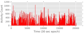
0 5000 10000 15000 20000 Time (30 sec epoch)

0 200 400 600 800 1000 1200

Activity Count

Figure 1: Activity time-series for a subject over a week.

be leveraged towards prediction tasks.

• A hierarchical model of representation:One of the per-sistent challenges in the time-series domain is the selection of time-segments granularity that serve as the primary analy-sis units. We explore learning representations at various lev-els of time granularity. We devise a novel algorithm that op-timizes two different measures to capture local and global patterns in the activity time-series, along with an ordinal loss to account for the natural ordering in the activities.

• Subject-invariant representations:The noise from the subjects environments can hinder generalization. In order to make the representations invariant to subject environments, we train our representations with a subject invariance loss.

Related Work

• Human activity for health informatics:Wearable sen-sors have mostly been used for human activity recogni-tion (HAR) task in machine learning (Bulling, Blanke, and Schiele 2014; Alsheikh et al. 2016), while medical practi-tioners perform a manual examination on the actigraphy data for diagnosing mostly sleep-disorders (Sadeh 2011). Recent works have tried using actigraphy data for quantifying sleep quality using deep learning (Sathyanarayana et al. 2016) or for actively monitoring human behavioral patterns (Althoff et al. 2017). The novelty of our method is that we propose task-agnostic models rather than plain supervised learning. • Representation learning: Bengio, Courville, and Vin-cent provide an overview of representation learning, used to construct a space that is discriminative for downstream tasks. It is based on ideas of better network convergence by adding (unsupervised) pre-trained vectors that encode the mutual information between the input features (Good-fellow, Bengio, and Courville 2016). Recently, the area has made enormous progress in NLP, vision, and speech (Col-lobert et al. 2011; Hinton et al. 2012). Of particular in-terest are the distributed bag-of-words (DBOW) architec-tures (Mikolov et al. 2013; Grover and Leskovec 2016; Saha et al. 2017) optimized to predict the context of the struc-ture, unlike continuous-bag-of-words (CBOW) that predicts the structure from its context. In a similar fashion, we use DBOW to capture local patterns in a time segment. Our nov-elty lies in integrating it in an adversarial setting (Ganin et al. 2016) with an unsupervised predictor, consisting of DBOW with global context and ordinal constraints.

• Time series analysis literature:These methods mainly use pair-wise similarity concept to perform classifica-tion (Bagnall et al. 2017) and clustering tasks, with

a distance metric like Euclidean. Dynamic Time Warp-ing (Berndt and Clifford 1994) is a widely used technique for finding similarity between two time-series which is compu-tationally expensive due to its pair-wise similarity approach. This has led to the creation of symbolic representation tech-niques like SAX (Lin et al. 2007) and BOSS (Sch¨afer 2015), that convert time-series into a symbolic sequence based on amplitudes or frequency analysis, respectively. SAX-VSM and BOSS-VS (Sch¨afer 2016) use tf-idf (term frequency-inverse document frequency) transformation of these sym-bolic sequences to get vector representation of sequence windows. HCTSA (Fulcher and Jones 2014) is an unsuper-vised time-series feature extraction engine with over 7800 feature space based on frequency-domain and time-domain analysis of the time-series, unlike the above supervised vec-tor space models. These time-series models, however, can-not complement the supervised learning model, unlike our model’s embeddings that can be used to initialize the archi-tectures with back-propagation like neural networks.

Our Approach

In this section, we describe our methodactivity2vec. We first describe challenges, followed by the model components that address these challenges.

Challenges for

activity2vec

To create a representational schema for activity time-series, the first natural challenge is determining the right granu-larityof the analysis unit. For example, consider the sample time-series in Figure 1, where the x-axis represents the time in 30 seconds epochs and the y-axis represents the activity levels, which in our setting are discrete values ranging from 0 to5000. Learning representations for each activity level might result in sparse vectors that are too fine-grained to be effective in the downstream tasks. Similarly, learning a rep-resentation with too big an analysis unit (e.g., spanning a week) could result in generic vectors lacking required dis-criminative power. As we demonstrate in our experiments, the right level of granularity is somewhere in between (a day span). Within the analysis units, therelative magnitudeof the signal values (e.g.,‘10’<‘15’) should accounted for.

Considering granularity of analysis unit shorter than the sequence length posits another challenge – how to cap-ture theglobal contextual dependenciesbetween the units. Since the units are parts of a sequence that describes a per-son’s activity over a timespan, they are likely to be inter-dependent which should be captured in the representations. The same activity can look very different across the subjects owing tosubject-specificnoise and environment,e.g.,how they wear the device on their wrist. Ouractivity2vecmodel addresses these challenges as described in the next section.

Problem Formulation and Time Granularity

Let S = {S1, S2,· · ·, SN} denote a set of activity

se-quences forP unique subjects, where each sequenceSn =

(t1, t2, . . . , tl) is l-length activity (e.g., step counts) for a

(3)

Tk Segmentation

Tk

Embedding Matrix

tj

Tk Ti

Smoothing

Tk

N(Tk)

Ordinal

Subject P

E

Segment Specific

F

Adversary Loss

D

E

F

Tk

D p

Neighbor Prediction

Softmax

Combined Loss

Figure 2: Graphical flow ofactivity2vec’s components: encoder E (embedding matrix), regularized predictors F, and the subject discriminator D. Figure on left shows the sub-losses of the three components, while figure on right shows the overall schema of a three-player game between F, D, and E. First, segmentation is done based on the time granularity. For a selected segment

Tk, its embeddingΦ(Tk)is first looked up from E. The embedding is then used by the predictors in F and the discriminator

D. The encoder E plays a cooperative game with F to allow it to induce the necessary information. E also plays an adversarial min-max game against D to prevent it from identifying the subject from the embedding to promote subject invariance.

to encode. We first break each sequenceSnintoK

consecu-tive time segments of equal length based ong(top of Figure 2). LetTk = (ta, ta+1, . . . , ta+L−1) ∈ T be such a

seg-ment of lengthLthat starts at timea. Our aim is to learn a mapping functionΦ:T →Rdto represent each time

seg-mentTkby addimensional representation. Equivalently, if

we represent each time segment in the dataset with a unique identifier (ID), the mapping functionΦis a lookup opera-tion on an embedding matrix of a single hidden layer neu-ral network with non-linear activations. Our goal is to learn the embedding matrix by considering the segment’scontent andcontextwhile promoting subjective invariance.Sn can

be obtained by concatenating (or averaging) theK segment-level vectors; we use concatenation. In this work, we con-sider the following time spans for a comparative analysis:

• Sample (sample2vec): representation for each 30-second sample. Our 20,160 length time-series yields a rep-resentation space ofR20160×d.

• Hour (hour2vec):representation for one-hour chunks, producing a vector space ofR168×d.

• Day (day2vec):embeds time-series at the level of a day span, giving us a representational space ofR7×d.

• Week (week2vec):provides embeddings at the scale of a week, yielding a vector inRdspace.

For a given granularity level,activity2vec learns the map-ping functionΦ. While it is possible to use a pre-processing step with change-points detection (CPD) to get the time-segments instead of manually setting the granularity, this step needs careful adjustments to set the thresholds for CPD models adding to further complexity of the model. In prin-ciple, we can have a space search over the possible granu-larities instead of using the pre-defined set above. We skip that step in this work for the sake of simplicity. Instead, we

demonstrate the model’s behavior for the choice of granu-larities that are intuitive to humans. Figure 2 presents the graphical flow ofactivity2vec.

Our model relates to the sequential methods like LSTM by taking into account the global temporal dependencies. Con-sidering the inter-segment and intra-segment context is anal-ogous to a shallow auto-encoder with very dense localized connections and sparse neighboring connections. While we leverage the discrete valued nature of our time-series, we can apply this method to continuous valued time-series by discretization, as done in the traditional time-series litera-ture. The adversarial setting motivated by the environmen-tal noise, which might not apply to other domains. We first present the loss components, and then the combined loss.

Modeling Segment Content in

activity2vec

We use two loss functions inactivity2vecto capture the con-tent of a segment – the ordinal relation between time-series values and their co-occurrence patterns.

Segment-Specific Loss We use the segment-specific loss to learn a representation for each time segment by pre-dicting its own values. Given an input sequence Tk =

(ta, ta+1, . . . , ta+L−1), we first map it to a unique vector Φ(Tk)by looking up the corresponding vector in the shared

embedding matrix Φ. We then use Φ(Tk)to predict each

symboltj sampled randomly from a window inTk.

How-ever, using a softmax layer for the prediction is very compu-tationally expensive. To compute the prediction loss in an ef-ficient manner, we use Noise-Contranstive Estimation (Gut-mann and Hyv¨arinen 2012) as an alternative to softmax:

Ls(Φ,Ws|Tk, tj) =−logσ(wt>jΦ(Tk)) (1)

−

M X

m=1

Etm∼ν(t)logσ(−w >

(4)

whereσis the sigmoid function defined asσ(x) = 1/(1 +

e−x_),_w

tj andwtm are the weight vectors associated with

tj andtmsymbols, respectively,ν(t)is the noise

distribu-tion from which negative exampletmis sampled, andM is

the number of negative examples sampled for each positive example. In our experiments, we use unigram distribution as the noise distribution withM = 12.

Since we ask the same segment-level vector to predict its symbols, the model captures the overall pattern of a seg-ment. Note that except forsample2vec, the model learns embeddings for both segments and symbols. A segment-based approach is commonly used in the time-series anal-ysis, though among the representational models only mod-els like SAX-VSM (Senin and Malinchik 2013) look at the co-occurrence statistics, with abag-of-wordsassumption.

Ordinal Regression Loss When predicting an activity symbol, the segment-specific loss above treats each symbol independently. However, since the symbols represent activ-ity levels, there is a natural ordering in their values (e.g.,‘5’

>‘1’), which should be preserved in representations. In or-der to embed this ordinal relation, we use ordinal regression loss while learning the representation for each activity value:

Lo(Φ, θ,wo|tj) =− V X

c=1

I(tj=c) log h

σ(θc−w

> oΦ(c))

−σ(θc−1−w>oΦ(c)) i

(2)

whereσ(x)is the sigmoid function as defined before,Iis

the indicator function, andV is the number of distinct dis-crete values that time-series can take (0-5000 in our case). Here,σ(θc−w>oΦ(c)) =p(tj ≤c|Φ(c))is the cumulative

probability oftj being at mostcwithθc being the ordered

threshold for the regression, such thatθj > θi,∀j > i. Remark:In principle, we can integrate the ordinal relation in Equation 1 with the NCE loss. However, owing to the hi-erarchical nature of our algorithm, the segment ID is also predicted while learning the symbols and segments repre-sentations. Since these segment-level IDs do not have an or-dinal relation with the symbol IDs, we resort to using an ordinal loss applicable only to time-series symbols.

Modeling Segment Context in

activity2vec

Loss functions presented above capture local patterns in a segment. However, since the segments are contiguous and describe activities of a person, they are likely to be related. For example, after a strenuous activity, there might be lighter activity periods. Likewise, one can expect a smooth tran-sition from one segment to the next. The algorithm should capture relations between proximal segments. With this mo-tivation, we use two loss functions to model this relationship.

Neighbor Context Loss Similar to activity symbols, each segment in the dataset is assigned a unique identifier that we can use to look up its corresponding vector in the em-bedding matrix or to predict the segment ID. We first for-mulate the relation between neighboring segments by ask-ing the current segment vectorΦ(Tk)(i.e.,looked-up vector

for segmentTk) to predict its neighboring segments in the

time-series:Tk−1andTk+1. If Ti is a neighbor toTk, the

neighbor context loss is the neighbor prediction task using NCE as before:

Lnc(Φ,Wnc|Tk, Ti) =−logσ(w>TiΦ(Tk)) (3)

−

M X

m=1

ETm∼ν(T)logσ(−w >

TmΦ(Tk))

where,wTiandwTm are the weight vectors associated with

Ti and Tm segments, respectively. The noise distribution

ν(T)is as described before over segment IDs.

Smoothing Loss While the previous objective attempts to capture neighborhood information, we also hypothesize that there is a “continuity” between neighboring segments. The learning algorithm should discourage any abrupt changes in the representation of proximal segments. We apply smooth-ing between the neighborsmooth-ing segmentsby minimizing thel2

-distance between representations of the neighbors:

Lr(Φ|Tk,N(Tk)) = η

|N(Tk)| X

Tc∈N(Tk)

kΦ(Tk)−Φ(Tc)k2

(4) where N(Tk)is the set of time-segments in proximity to

Tkandηis the smoothing strength parameter. Note that the

smoothing loss is not applicable toweek2vec.

Modeling Subject Invariance in

activity2vec

One challenge in dealing with human activity data is that it heavily depends on the subject’s environment. To promote subject invariance, we use anadversary loss (Ganin et al. 2016). LetP be the number of unique subjects. We use a multi-class classifier as adiscriminatorto predict the time-segment’s source (subject)s∈ {1, . . . , P}from the encoded segment representationΦ(Tk). In other words, the

discrim-inator tries to identify the subject from whose activity time-series the encoder(the embedding matrix) has derived the segment’s representation. Note that we want to emphasize the invariance from the source subject of the time-segment and not from the particular sequence from which the seg-ment is derived. Hence, if we have multiple sequences for the same subject, the sequences will share the same subject

sin our model. Formally, the discriminator is defined by a soft-max:

p(s=p|Φ(Tk),U) =

exp(uT

pΦ(Tk))

P

p0exp(uT_p0Φ(Tk))

(5)

whereupis the weight vector associated with subjectp, and

Udefines all the parameters of the discriminator. We use a cross-entropy loss to optimize the subject discriminator:

Ld(U|Φ, Tk, s=p) =− P X

s=1

I(s=p) logp(s=p|Φ(Tk),U) (6)

wherepis a subject from whom the segmentTkis encoded.

With a goal to promote subject invariance, we put the en-coder (the embedding matrix) in adversary with the discrim-inator. The encoder attempts to encode features that are in-distinguishable to the subject discriminator by minimizing (negative of discriminator loss):

La(Φ|U, Tk, s=p) = P X

s=1

(5)

Combined Loss for

activity2vec

We define ouractivity2vecmodel as the combination of the losses described in Equations 1, 2, 3, 4, and 7:

L(Φ) =

N X

n=1

X

Tk∈Sn

X

tj∈Tk Ti∈N(Tk)

h

Ls(Φ,W|Tk, tj) +βLo(Φ, θ,wo|tj)

| {z }

Segment Content

+

Lnc(Φ,W|Tk, Ti) +Lr(Φ|Tk,N(Tk))

| {z }

Segment Context

+λLa(Φ|U, Tk, s)

| {z }

Adversarial

i

(8) whereβ >0andλ >0are the relative weights for the or-dinal regression loss and the subject invariance loss, respec-tively. Concurrently, we also minimize the discriminator loss in Equation 6. As shown at the right in Figure 2, the training ofactivity2vecinvolves an optimization game between three players: the encoder (E), the combined predictor (F), and the discriminator (D). E plays a cooperative game with F to al-low it to induce the necessary information. E also plays an adversarial min-max game against D to prevent it from iden-tifying the subject from the encoded vector to promote sub-ject invariance. We train our model using stochastic gradient descent (SGD).

The main challenge in adversarial training is to balance the two components – the combined loss in Eq. 8 vs. the discriminator loss in Eq. 6, as shown (right) in Figure 2. If one player becomes smarter, its loss to the shared encoder (embedding matrix) overwhelms, and the training fails to converge (Arjovsky, Chintala, and Bottou 2017). In our ex-periments, the discriminator converges much faster. To sta-bilize the training, we update the discriminator once every five gradient steps of the algorithm, chosen randomly. Also, we follow the weighting schedule proposed by (Ganin et al. 2016, p. 21), that initializesλto0, and then changes it grad-ually to1 as training progresses. Through our experiments we demonstrate that the intuitions captured by the compo-nents are synergistic since they improve the performance in-crementally as the components are added.

Experimental Settings

In this section, we describe experimental settings — datasets, the prediction tasks on which we evaluate the em-beddings, the baselines models, and parameter selection.

Datasets

We use Study of Latinos (SOL) (Sorlie et al. 2010) and Multi-Ethnic Study of Atherosclerosis (MESA) (Bild et al. 2002) datasets. SOL has physical activity and clinical data for 1887 subjects, while MESA only has activity data for 2237 subjects. This simulates the scenario where disorder condition labels are available only for a portion of users. These datasets contain activity data (actigraphy) from each subject for a minimum of 7 days measured with wrist-worn Philip’s Actiwatch Spectrum. The time-series for each sub-ject is sampled at a rate of 30 seconds. Actigraphy records the mean activity count reported with ZCM (Zero Crossing Mode) per 30 seconds, providing us with a signal that can only take integer values. This makes embedding the input symbols straightforward, without any pre-processing. The

few missing values (< 1%) observed in the data-set were replaced by unknown (UNK) token. The datasets are not skewed with respect to the class distribution of different pre-diction tasks described next.

Prediction Tasks

We evaluate the effectiveness of the learned embeddings on the following health disorder prediction tasks:

• Sleep Apnea:Sleep apnea syndrome is a sleep disorder characterized by reduced respiration during the sleep time. We use the Apnea-Hypopnea Index (AHI) at 3% desatura-tion level with AHI<5 being characterized asnon-apneaic, while AHI>5indicating amild-to-severe-apnea.

• Diabetes: Diabetes (type 2) is the body’s insensitivity to insulin, leading to elevated levels of blood sugar. Task is defined as a three-class classification problem, to decide whether a subject is anon-diabetic,pre-diabetic, ordiabetic.

• Hypertension: Hypertension refers to abnormally high levels of blood pressure, an indicator of stress. Hyperten-sion prediction characterizes a binary classification problem for increased blood pressure.

• Insomnia:Insomnia is a sleep disorder characterized by an inability to fall asleep easily, leading to low energy lev-els during the day. We use a 3-class prediction problem for classifying subjects intonon-,pre-andinsomniacgroups.

Baseline Models

We compare our method with a number of naive baselines and existing systems that use time-series representations: (a) Majority Class:This baseline always predicts the class that is most frequent in a dataset.

(b) Random:This baseline randomly picks a class label. (c) SAX VSM: SAX-VSM (Senin and Malinchik 2013) uses SAX, one of the most widely used time-series repre-sentation technique.

(d) BOSS:BOSS (Sch¨afer 2015) is a symbolic representa-tional learning technique that uses Discrete Fourier Trans-form (DFT) of time-series windows. BOSS creates equal sized bins from histograms of DFT coefficients, which are then assigned representational symbols. Labels are assigned based on the class that gets the highest similarity score using nearest neighbor approach.

(e) BOSSVS:BOSS in Vector Space (Sch¨afer 2016) is sim-ilar to SAX-VSM and creates vector space representation of the time-series from BOSS. BOSS is known to be one of the most accurate methods on standard time-series classification tasks, with BOSS-VS performing marginally lower. (g) CNN:We use a Convolutional Neural Network (CNN) with Conv-ReLU-AvgPool-BatchNorm-Dropout layers for supervised prediction. We add layers until we get no per-formance improvement on held-out set.

(6)

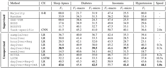
Table 1:F1andSpeedrelative towall clock timeof ourday2vec+Reg+O+A. O refers toOrdinal and A toAdversarial.

Method Clf. Sleep Apnea Diabetes Insomnia Hypertension Speed

F1 F1-macro F1-micro F1-macro F1-micro F1

Super

vised

Majority 0-R 00.0 21.7 31.9 47.4 25.5 00.0

-Random 33.9 34.3 31.3 36.2 30.0 33.4

-SAX-VSM 00.0 38.6 24.3 47.4 25.5 00.0

-BOSS 17.6 38.9 31.5 49.8 34.9 29.6

-BOSSVS 11.7 40.1 32.7 47.5 33.1 31.3

-Task-specific CNN 41.5 45.2 41.0 50.7 40.1 36.6 2.0x

Unsuper

vised

sample2vec LR 36.7 40.0 36.7 42.4 35.3 39.4

-hour2vec LR 30.0 41.4 33.3 44.6 28.5 24.4

-hour2vec+Reg LR 20.5 42.1 32.0 43.5 28.7 23.1

-day2vec LR 36.8 40.9 38.0 45.2 35.8 40.3 0.3x

day2vec+Reg LR 38.9 41.8 39.5 46.6 39.7 43.4 0.3x

week2vec LR 14.5 40.6 34.1 44.2 31.5 18.7

-HCTSA LR 20.3 40.0 35.0 46.7 33.7 22.0 8.2x

LSTM LSTM 32.2 41.4 33.3 46.1 30.4 37.8 10.5x

day2vec+Reg+O LR 40.5 45.3 40.2 50.9 40.3 43.6 0.4x

day2vec+Reg+O+A LR 43.6 45.8 42.5 55.7 41.4 44.1 1.0x

(i) LSTM: We train an LSTM based unsupervised model similar to (Sundermeyer, Schl¨uter, and Ney 2012) that learns to encode sequences by predicting next time-series value (as a language model in NLP). Next, we use this pre-trained net-work to initialize the LSTM netnet-work that is further trained on the supervised learning tasks.

Variants ofactivity2vec (a) Unregularized models:This group of models contain only two NCE loss components from Equation 8: Ls and Lnc. In the Results section,

we refer to these models as sample2vec, hour2vec, day2vec, andweek2vec.

(b) Regularized models: We add smoothing loss Lr to

models in (a). This group includes hour2vec+Regand day2vec+Reg. We omit sample2vec+Reg since it performed extremely poorly on all the tasks. Recall that smoothing is not applicable toweek2vec.

(c) Ordinal loss model:We use ordinal lossLowith these

models. We add this loss today2vec+Regmodel in (b), our best performing model as discussed in the next section. We omit other time-unit models for brevity.

(d) Adversarial model: These models use the adversary lossLafor ourday2vec+Regwith ordinal loss.

Hyper-Parameter Selection

We use 80%,10%,10% split for train, validation, and test sets repeated 10 times, and we report the mean scores. As mentioned earlier, we only have the disorder task labels for the SOL dataset. For the supervised models we only use the SOL dataset, while for the unsupervised models we use the combined SOL and MESA data. The embedding size ofd=100was fixed for all the models. The weighting parameters λ and β were chosen to be 0.05 and 0.5, re-spectively. The remaining hyper-parameters inactivity2vec are: window size (w) for segment-specific loss, number of neighboring segments (|N(Tk)|) and regularization strength

(η) for day2vec and hour2vec. We tuned for w ∈ {12,20,30,50,100,120,500},η ∈ {0,0.25,0.5,0.75,1}, and|N(Tk)| ∈ {2,4}on the development set. We chosew

of size 20, 20, 30, and 50 forsample2vec,hour2vec, day2vec, andweek2vec, respectively. Theηof 0.25 and 0.5 were chosen for day2vec and hour2vec,

respec-tively. The neighbor set size of 2 was chosen. For the CNN baseline, 3, 4, 3, and 3-layered network were used for sleep-apnea, diabetes, insomnia, and hypertension, with a dropout of 0.5 trained with Adam Optimizer. We tuned all the pa-rameters for maximizing theF1scores.

Results and Discussion

In this section, we present our results for the four pdiction tasks described in the previous section. The re-sults are presented in Table 1 in four groups: (i) baselines, (ii) existing time-series representation methods and CNN, (iii) our unregularized and regularizedactivity2vecvariants, and (iv) our ordinal and adversarialactivity2vecmodels. We show classification performance in terms ofF1scores.

• Performance on disorder classification tasks:Since our goal is to evaluate the effectiveness of the learned vectors, we use simple linear classifier Logistic Regression (LR) with our activity2vec models. For the multi-class classifi-cation problems like Diabetes and Insomnia, we use One-vs-All classifiers, tuning for micro-F1 score. We run each

experiment 10 times and take the average of the evaluation measures to avoid any randomness in results. We can notice that day2vec consistently gives absolute 2-4% improve-ments over the otheractivity2vecvariants, and 6-20% over the baseline time-series representation models and LSTM on

F1 scores on all tasks. The adversarial-ordinal-regularized

variant of day2vec gives the best results among all the variants. Adversarial variant performs at par or better than task-specific supervised CNN on all the tasks. Due to inher-ent noisy nature of activity time-series and long sequence length, the LSTM-based model did not work well.

(7)

pro-10 25 50 75 100 Amount of Training Labels (%) 25.0

27.5 30.0 32.5 35.0 37.5 40.0 42.5

Test F1 Score

Sleep Apnea

CNN day2vec+LR

10 25 50 75 100 Amount of Training Labels (%) 30

32 34 36 38 40 42 44

Test Micro-F1 Score

Diabetes

CNN day2vec+LR

34 36 38 40

Test Micro-F1 Score

Insomnia

CNN day2vec+LR

25 30 35 40 45

Test F1 Score

Hypertension

CNN day2vec+LR

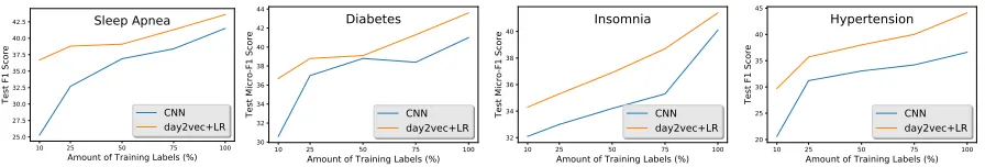
Figure 3: Comparison of our unsupervisedday2vec+Reg+O+Awith LR vs. supervised CNN as a function of labeled data.

duces marginally better results than thesample2vec de-spite much lower dimensional space (2880x). The level of granularity makes a lot of difference in the performance of our models. From the above results, we can conclude that while the low granularity level (sample2vec) suffered from coarse embeddings, the high granularity (week2vec) level embeddings lost the ability to discriminate.

• Effect of smoothing:Intuition behind adding the tempo-ral smoothing loss (Eq. 4) to our model was to test the hy-pothesis that human activities happen in continuity and fol-low a macro-routine. This should be reflected in neighbor-ing time-segments makneighbor-ing them similar in structure. As re-sults suggest, the continuity hypothesis was misguided at the sample- and hour-level. Regularization at the sample level made them lose the discriminative power for classification— considering the noise in activity levels at such a fine gran-ularity.hour2vec+Regexhibits a significant drop (sleep apnea) or at par performance compared to hour2vec. Since humans tend to switch between different activity types at the order of hours or less, the hypothesis of continuity was inappropriate at hour level as well. However, adding smooth-ing helps produce gains forday2vec, our best model. We argue that smoothing regularization helps capture a higher level global context since humans structureroutines at the level of the day, while we switch between activities on the order of hours or lower. This is supported by the peri-odogram analysis, where day level frequencies dominate.

• Effect of ordinal loss:Addition of ordinal loss improves the accuracy of our models, albeit marginally. While the other loss functions work on co-occurrence of activity values at local and global contexts, ordinal loss explicitly models the relationship between the magnitude of the activity val-ues,e.g.,‘25’>‘5’. While it can be argued that similar ordi-nal values would co-occur, hence reflected in theLs, adding

Figure 4: t-SNE visualization of subjects with regularized day2vecon the left and adversarialday2vecon the right, for all the subjects with respect to their level of activity.

an explicit ordinal constraint helps, though marginally.

• Effect of adversarial training: Adding the adversarial loss to the ordinal-regularized models improves the F1

scores across the tasks by 0.5%-3.1% in absolute numbers and 2%-7.5% in relative terms. The difference in perfor-mance is more than the 95% confidence intervals around the repeated experimental means reported here. It can thus be concluded that making the representations invariant to the source (subjects) helps in removing the noise introduced by the subjects and their environments, owing to how they wear their device and their routines, making the embeddings more generalized. With an adversarial setting, we can create a rep-resentation space more relevant to the health condition of the subjects by removing the subject source domain.

Figure 4 shows the t-SNE (Maaten and Hinton 2008) plot of regularized day2vec(left) vs adversarialday2vec em-beddings (right) for SOL dataset subjects. For each subject, we concatenate the embeddings from constituent day level time-segments. We plot the lifestyles of the subjects as deter-mined by the study questionnaire, identifying each subject as highly-active, moderately-active, and sedentaryperson. We can notice clusters or subjectphenotypeswith nice sep-aration within the cluster for each of the lifestyle type with non-adversarialday2vec. Unsurprisingly, the clusters get very compact in the adversarial setting. The lifestyle classes get clustered markedly separately rather than forming in-cluster separations, observed in the non-adversarial setting. Hence, the adversary helpsactivity2vecwith removing the subject-wide variance in the learned embeddings, while still capturing the properties of subject phenotypes. Also, adver-sary loss improved results on the disorder prediction tasks. Hence, by reducing subject level variance, the adversary loss helps encode a better global representation.

• Scalability:Our model (Table 1) takes much less training time compared to the deep unsupervised model like LSTM. In fact, our model takes much less time compared to the supervised CNN that only runs on the labeled data. Since our model has only one hidden layer (i.e.,embedding layer) and uses NCE for training, it is scalablein practical set-tings compared to the deep neural models. Additionally, our model offers moreflexibilityto incorporate the alternative intuitions including human knowledge (e.g., the day/hour level representational hierarchy) that would be difficult to do with other deep methods. Clearly, using more sophis-ticated deep neural models like deep auto-encoders for a semi-supervised setting would pose scalability challenges.

(8)

representations for unseen segments can be derived by a sin-gle backprop step (Le and Mikolov 2014).

• Supervised vs Unsupervised:To show the utility of un-supervised schema, we demonstrate the performance of su-pervised CNN vs. our adversarial day2vec method as a function of the percentage of labeled data in Figure 3. Clearly, our model outperforms CNN across the board. The gap is drastic when the proportion of labeled data is low, which is usually the case in practice.

Conclusions

In this work, we present a novel unsupervised representa-tional learning technique,activity2vecthat encodes human activity time-series by modeling local and global activity patterns. We train our model on two datasets and test on pre-diction tasks (four commonly occurring disorders). We find that day-level granularity preserves the best representations, which is not surprising since a day is a natural timescale for a full cycle of human activities. Our task-agnostic represen-tational learning model using simple linear classifiers beats baseline time-series representation models on all the disor-der prediction tasks. It even performs at par or better than su-pervised convolutional neural network baseline. Our model learns the representational features using a combination of non-linear loss functions, giving better performance on mul-tiple tasks using simple linear classifiers. We further demon-strate that using adversarial loss along with our embedding encoder model helps increase the performance and gener-alizability of the embeddings. Additionally, our method is capable of complementing the supervised learning by ini-tialization, unlike existing representation approaches.

References

Alsheikh, M. A.; Selim, A.; Niyato, D.; Doyle, L.; Lin, S.; and Tan, H.-P. 2016. Deep activity recognition models with triaxial accelerometers. InAAAI Workshops.

Althoff, T.; Horvitz, E.; White, R. W.; and Zeitzer, J. 2017. Har-nessing the web for population-scale physiological sensing: A case study of sleep and performance. InWWW, 113–122.

Arjovsky, M.; Chintala, S.; and Bottou, L. 2017. Wasserstein GAN. CoRRabs/1701.07875.

Bagnall, A.; Lines, J.; Bostrom, A.; Large, J.; and Keogh, E. 2017. The great time series classification bake off: a review and experimental evaluation of recent algorithmic advances. DMKD 31(3):606–660.

Bengio, Y.; Courville, A.; and Vincent, P. 2013. Representation learning: A review and new perspectives. TPAMI 35(8):1798– 1828.

Berndt, D. J., and Clifford, J. 1994. Using dynamic time warping to find patterns in time series. InKDD workshop, volume 10, 359– 370. Seattle, WA.

Bild, D. E.; Bluemke, D. A.; Burke, G. L.; Detrano, R.; Diez Roux, A. V.; Folsom, A. R.; Greenland, P.; JacobsJr, D. R.; Kronmal, R.; Liu, K.; et al. 2002. Multi-ethnic study of atherosclerosis: objec-tives and design. American journal of epidemiology156(9):871– 881.

Bulling, A.; Blanke, U.; and Schiele, B. 2014. A tutorial on human activity recognition using body-worn inertial sensors.ACM CSUR 46(3):33.

Collobert, R.; Weston, J.; Bottou, L.; Karlen, M.; Kavukcuoglu, K.; and Kuksa, P. 2011. Natural language processing (almost) from scratch. JMLR12(Aug):2493–2537.

Fulcher, B. D., and Jones, N. S. 2014. Highly comparative feature-based time-series classification.TKDE26(12):3026–3037. Ganin, Y.; Ustinova, E.; Ajakan, H.; Germain, P.; Larochelle, H.; Laviolette, F.; Marchand, M.; and Lempitsky, V. 2016. Domain-adversarial training of neural networks. JMLR17(1):2096–2030. Goodfellow, I.; Bengio, Y.; and Courville, A. 2016.Deep Learning. MIT Press.

Grover, A., and Leskovec, J. 2016. node2vec: Scalable feature learning for networks. InACM SIGKDD, 855–864.

Gutmann, M. U., and Hyv¨arinen, A. 2012. Noise-contrastive es-timation of unnormalized statistical models, with applications to natural image statistics.JMLR 201213(Feb):307–361.

Hinton, G.; Deng, L.; Yu, D.; Dahl, G. E.; Mohamed, A.-r.; Jaitly, N.; Senior, A.; Vanhoucke, V.; Nguyen, P.; Sainath, T. N.; et al. 2012. Deep neural networks for acoustic modeling in speech recog-nition: The shared views of four research groups.IEEE Signal Pro-cessing Magazine29(6):82–97.

Le, Q., and Mikolov, T. 2014. Distributed representations of sen-tences and documents. InICML, 1188–1196.

Lin, J.; Keogh, E.; Wei, L.; and Lonardi, S. 2007. Experiencing sax: a novel symbolic representation of time series.DMKD15(2):107– 144.

Maaten, L. v. d., and Hinton, G. 2008. Visualizing data using t-sne. JMLR9(Nov):2579–2605.

Mikolov, T.; Sutskever, I.; Chen, K.; Corrado, G. S.; and Dean, J. 2013. Distributed representations of words and phrases and their compositionality. InNIPS, 3111–3119.

Sadeh, A. 2011. The role and validity of actigraphy in sleep medicine: an update.Sleep medicine reviews15(4):259–267. Saha, T. K.; Joty, S.; Hassan, N.; and Hasan, M. A. 2017. Regu-larized and retrofitted models for learning sentence representation with context. InCIKM, 547–556. ACM.

Sathyanarayana, A.; Joty, S.; Fernandez-Luque, L.; Ofli, F.; Srivas-tava, J.; Elmagarmid, A.; Taheri, S.; and Arora, T. 2016. Impact of physical activity on sleep: A deep learning based exploration. arXiv preprint arXiv:1607.07034.

Sch¨afer, P. 2015. The boss is concerned with time series classifi-cation in the presence of noise.DMKD29(6):1505–1530. Sch¨afer, P. 2016. Scalable time series classification. DMKD 30(5):1273–1298.

Senin, P., and Malinchik, S. 2013. Sax-vsm: Interpretable time series classification using sax and vector space model. InICDM, 1175–1180. IEEE.

Sorlie, P. D.; Avil´es-Santa, L. M.; Wassertheil-Smoller, S.; Kaplan, R. C.; Daviglus, M. L.; Giachello, A. L.; Schneiderman, N.; Raij, L.; Talavera, G.; Allison, M.; et al. 2010. Design and implementa-tion of the hispanic community health study/study of latinos. An-nals of epidemiology20(8):629–641.

Storm, F. A.; Heller, B. W.; and Mazz`a, C. 2015. Step detection and activity recognition accuracy of seven physical activity monitors. PloS one10(3):e0118723.

Sundermeyer, M.; Schl¨uter, R.; and Ney, H. 2012. Lstm neural networks for language modeling. InINTERSPEECH.