Adaptive Proximal Average Based Variance Reducing Stochastic Methods for Optimization with Composite Regularization

(1)

The Thirty-Third AAAI Conference on Artificial Intelligence (AAAI-19)

Adaptive Proximal Average Based Variance Reducing

Stochastic Methods for Optimization with Composite Regularization

Jingchang Liu, Linli Xu, Junliang Guo, Xin Sheng

School of Computer Science and Technology

University of Science and Technology of China, Hefei, China

[email protected], [email protected],{guojunll, xins}@mail.ustc.edu.cn

Abstract

We focus on empirical risk minimization with a composite regulariser, which has been widely applied in various ma-chine learning tasks to introduce important structural infor-mation regarding the problem or data. In general, it is chal-lenging to calculate the proximal operator with the composite regulariser. Recently, proximal average (PA) which involves a feasible proximal operator calculation is proposed to approx-imate composite regularisers. Augmented with the prevail-ing variance reducprevail-ing (VR) stochastic methods (e.g. SVRG, SAGA), PA based algorithms would achieve a better per-formance. However, existing works require a fixed stepsize, which needs to be rather small to ensure that the PA approx-imation is sufficiently accurate. In the meantime, the smaller stepsize would incur many more iterations for convergence. In this paper, we propose two fast PA based VR stochas-tic methods – APA-SVRG and APA-SAGA. By initializing the stepsize with a much larger value and adaptively decreas-ing it, both of the proposed methods are proved to enjoy the

O(nlog1 +m0

1

) iteration complexity to achieve the

-accurate solutions, wherem0 is the initial number of inner

iterations andnis the number of samples. Moreover, exper-imental results demonstrate the superiority of the proposed algorithms.

Introduction

In many artificial intelligence and machine learning applica-tions, one needs to solve the following generic optimization problem in the form of regularized empirical risk minimiza-tion (ERM) givennsamples (Hastie, Tibshirani, and Fried-man 2001):

min

x∈Rd

F(x) := 1 n

n

X

i=1

fi(x) +r(x), (1)

wherefi : Rd → Rdenotes the empirical loss of thei-th

sample with regard to the parameterx, andris the regular-ization term, which is convex but possibly non-smooth. The goal is to find the optimal solution ofxthat minimizes the regularized empirical loss over the whole dataset.

To solve the problem, deterministic algorithms including traditional gradient descent (GD) and accelerated gradient descent (AGD) (Nesterov 2013) are proposed, which involve

the calculation ofngradients. When the data size scales up,

n can be rather large, which makes the calculation in de-terministic algorithms unaffordable. An effective alternative is stochastic gradient descent (SGD) (Robbins and Monro 1951) which involves lower per iteration cost by utilizing the stochastic gradient instead of the full gradient to updatex. However, a rather large variance introduced by the stochas-tic gradient would slow down the convergence (Bottou, Cur-tis, and Nocedal 2016). To address this issue, a number of variance reducing (VR) stochastic methods are proposed re-cently, including SAG (Schmidt, Le Roux, and Bach 2017), SVRG (Johnson and Zhang 2013), SAGA (Defazio, Bach, and Lacoste-Julien 2014) and SARAH (Nguyen et al. 2017). As the key feature of these methods, the variance of stochas-tic gradient asymptostochas-tically goes to zero along the iterative updates, which allows them to achieve the linear conver-gence rate when each loss is supposed to be strongly convex. To obtain a compact representation of models, non-smooth regularisers are often used in regularized ERM prob-lems. Based on the VR stochastic methods mentioned above, a general routine for this case is to employ the forward-backward splitting (Singer and Duchi 2009), which involves the calculation of the proximal operator ofr, i.e., proxγ

r(·).

A formal definition of proxγ_r(·)is proxγ_r(x) =arg min

y∈Rd

r(y) + 1

2γky−xk

2

, (2)

whereγ > 0. One requirement for using proximal opera-tors is that proxγ

r(·) can be calculated effectively, such as

whenr(x) = kxk1. But in a large number of important ap-plications in machine learning, such as overlapping group lasso (Jacob, Obozinski, and Vert 2009) and graph-guided fused lasso (Kim and Xing 2009), the regularisers that take a composite formr(x) =PK

k=1wkrk(x)cannot be handled

(2)

and Gidel 2018; Pedregosa, Fatras, and Casotto 2018), but they make a strong assumption thatris smooth in the anal-ysis of strongly convex case.

An alternative to the above methods is to smooth the non-smooth regulariser. One traditional way is to utilize Nes-terov’s smoothing technique (Nesterov 2005; Chen et al. 2012). While recently, Yu (Yu 2013) introduces the proximal average (PA) approximation in accelerated proximal gradi-ent methods (PA-APG), and strictly shows its superiority over the smoothing techniques. Several works have further developed the PA method with different settings. Among them, (Yu et al. 2015) and (Zhong and Kwok 2014) apply the PA approximation to non-convex regularisers. (Zhong and Kwok 2014) combines PA with stochastic gradient methods. Further, PA is introduced to VR stochastic methods by (Che-ung and Lou 2017).

On the other hand, approximating a composite regulariser with PA would introduce approximation bias which is pro-portional to the stepsize according to (Yu 2013), and a small stepsize is required to ensure the accuracy of approximation. In (Yu 2013) and (Cheung and Lou 2017), a fixed stepsize is adopted and set as small asO(), where is the precision given in advance. This makes the algorithms impractical when a higher-precision solution is required. To tackle this issue, the adaptive stepsize strategy is introduced in (Zhong and Kwok 2014) and (Shen et al. 2017). Instead of setting the stepsize rather small at the beginning, algorithms with adaptive stepsize start with a large stepsize and reduce it gradually. In the two works mentioned above, the stepsize decreases at a rate of O(1/k), where k is the number of iterations. As a result, these algorithms enjoy significantly fewer iterations than the corresponding fixed stepsize algo-rithms when one needs a higher-precision solution.

In this paper, we apply the adaptive stepsize strategy to the PA-based VR stochastic algorithms, and propose the fol-lowing algorithms correspondingly: SVRG and APA-SAGA. Both algorithms consist of two layers of loops, the stepsize iteratively decreases toρ(0< ρ <1)times of the previous stepsize before the inner loop starts. Meanwhile, the number of inner loops inside each outer loop increases accordingly. We prove that the overall number of gradi-ent calculations of the proposed algorithms, APA-SVRG and APA-SAGA, are both O(nlog1 +m01) to achieve

-accurate solutions, wherem0 is the initial number of in-ner iterations. Note that such rate is superior to that of PA-ASGD in (Zhong and Kwok 2014). Compared to PA-based VR stochastic methods with fixed stepsize in (Cheung and Lou 2017), the proposed algorithms need significantly fewer iterations to achieve higher-precision solutions. On the other side, compared to ADMM-based VR stochastic algorithms, the proposed algorithms have low storage requirement as they do not need to store the transformation matrix, and are easier to implement and analyse. The experiments on over-lapping group lasso and graph-guided lasso empirically val-idate the superiority of proposed algorithms.

The rest of this paper is organized as follows. After in-troducing the problem formulation, assumptions used in the paper and reviewing the relevant theories of VR stochastic methods and proximal average, we respectively present the

proposed APA-SVRG and APA-SAGA algorithms, together with the corresponding convergence rate analysis. We then present the experimental results and conclude the paper.

Notation.In this paper, we denote the gradient of the differ-entiable functionfiatxas∇fi(x).kxkandkxk1are thel2 andl1norm of vectorxrespectively.h·,·idenotes the inner product.x∗denotes the point on whichFattains its optimal value, which is denoted byF∗. We usexkforxin thek-th iteration._E[·]denotes an expected value taken with respect to all choices of indexes up to the current iteration, while E[·]

denotes the expected value taken with respect to the choice of index at the current iteration.

Background and Related Work

In this section, we formulate the problem considered in this paper, together with some common assumptions. Then we overview the theories of variance reducing (VR) stochastic methods and proximal average (PA) which are the founda-tion of our methods.

Problem Formulation

We consider the following optimization problem

min

x∈Rd

F(x) =f(x) +r(x) = 1 n

n

X

i=1

fi(x) + K

X

k=1

wkrk(x),

(3) where wk ≥ 0 and PK_k₌₁wk = 1. The above

formula-tion defines a general regularized ERM, in which the reg-ulariser r is a convex combination of the K components

rk (k = 1,2, . . . , K). Such composite regularisers have

shown the superiority in capturing important structural in-formation regarding the problem or data, such as structured sparsity (Zhao, Rocha, and Yu 2009). The following lists the composite forms ofrfor two representative machine learn-ing models.

• Overlapping group lasso (Jacob, Obozinski, and Vert 2009). To select meaningful groups of features, the over-lapping group lasso is introduced with the regulariser

r(x) =λ

K

X

k=1

kxgkk, (4)

whereλ >0, andgkindicates the index group of features,

andxgkis the corresponding subvector ofx.

• Graph-guided fused lasso(Kim and Xing 2009). Graph-guided fused lasso leads to structured sparsity according to the graph G ≡ {V,E}, in whichV = {x1, . . . , xd},

wherexi ∈ R, is the vertex set andE is the set of edges

amongV. The regulariser is

r(x) = X {i,j}∈E

wij|xi−xj|, (5)

which would penalize the difference among variables con-nected inG.

To facilitate the analysis, we make the following assump-tions onfi’s and rk’s, which are common in optimization.

(3)

Assumption 1. EachfiisL-smooth (L > 0), namely for

anyx, y∈Rd,

fi(y)≤fi(x) +h∇fi(x), y−xi+

L

2ky−xk

2_. (6)

We also assume the strong convexity offi. This

assump-tion can be readily satisfied by combing the general convex loss functions with the strongly convex penalties, such as`2 norm.

Assumption 2. Each fi is µ-strongly (µ > 0) convex,

namely for anyx, y∈Rd,

fi(y)≥fi(x) +h∇fi(x), y−xi+

µ

2ky−xk

2_. ₍₇₎

For each non-smooth penaltyrk, we assume it to be

Lips-chitz continuous withLkas shown in the following

assump-tion.

Assumption 3. EachrkisLk-Lipschitz continuous, namely

for anyx, y∈Rd,

|rk(x)−rk(y)| ≤Lkkx−yk. (8)

Variance Reducing Stochastic Methods

The variance of stochastic gradient would limit the per-formance of stochastic algorithms. To effectively reduce the variance, some methods which employ the control variates (Owen 2013, Chapter 8.9) are introduced in re-cent years (Johnson and Zhang 2013; Defazio, Bach, and Lacoste-Julien 2014; Defazio, Domke, and others 2014; Schmidt, Le Roux, and Bach 2017). Among them, SVRG (Johnson and Zhang 2013) and SAGA (Defazio, Bach, and Lacoste-Julien 2014) are two representatives, which propose the following VR stochastic gradient:

vk=∇fj(xk)− ∇fj(˜x) +

1 n

n

X

i=1

∇fi(˜x), (9)

where ˜x is the retained ‘snapshot’ of x to replace the stochastic gradient∇fj(xk) in SGD. As the control

vari-ate of ∇fj(x), ∇fj(˜x) will asymptotically get closer and

closer to∇fj(x)in expectation along the iterative updates,

in which case the variance goes to zero. As a result, both SVRG and SAGA can converge under the fixed stepsize, and a large stepsize leads to a much faster convergence rate. Equipped with proximal operators to handle the nonsmooth regularisers, the corresponding algorithms are known as Prox-SVRG (Xiao and Zhang 2014) and Prox-SAGA (De-fazio, Bach, and Lacoste-Julien 2014), which involve the following update

xk+1=proxγ_r(xk−γvk), (10) whereγ >0is the fixed stepsize. When the regularizationr

is simple and admit an efficient proximal operation, Prox-SVRG and Prox-SAGA perform quite well both in prac-tice and theory. Next, we briefly review Prox-SVRG and Prox-SAGA together with the corresponding theories, which would be useful when establishing our own work.

Prox-SVRG consists of two loops. It savesx˜ and calcu-lates the full gradientPn

i=1∇fi(˜x)/njust before the inner

loop begins.x˜is kept in fixed number of iterations, and up-dated again just after the current outer loop ends.

The convergence analysis of Prox-SVRG under Assump-tion 1 and AssumpAssump-tion 2 is established in (Xiao and Zhang 2014). Define

θ= 1

γµ(1−4Lγ)m +

4Lγ(m+ 1)

(1−4Lγ)m, (11)

whereγis the stepsize andmis the number of inner loops inside each outer loop. Further denotex˜s=P

m

k=1xk/min

thes-th outer loop. The change of function value after one outer loop of Prox-SVRG is described as

EF(˜xs)−F∗≤θ[F(˜xs−1)−F∗]. (12) Therefore, if0 < γ <1/(4L)andmis large enough such thatθ <1, the linear convergence rate of Prox-SVRG with respect to the outer iterations can be obtained immediately.

Meanwhile in Prox-SAGA, a table is established to record the gradient∇fi(xi)for eachi= 1,2, . . . , n, herexi∈Rd

is the value ofxat one previous iteration. In this way, at the cost of memory consumption, Prox-SAGA is simpler as it avoids the expensive calculation of the full gradient.

The corresponding theories regarding the convergence of Prox-SAGA under Assumption 1 and Assumption 2 are es-tablished in (Defazio, Bach, and Lacoste-Julien 2014). The analysis is based on the Lyapunov function

Tk = 1 n

n

X

i=1

fi(xki)−f(x∗)−

1 n

n

X

i=1

∇fi(x∗), xki −x∗

+ckxk−x∗k2_. ₍₁₃₎

Then the relation betweenTk andTk+1can be set up:

E[Tk+1]−Tk≤ −1

κT

k₊_C

1 h

f(xk)−f(x∗)−

∇f(x∗), xk−x∗i

+C2 h1

n

X

i=1

fi(xki)−f(x ∗

) +1

n

X

i=1

∇fi(x ∗

), xk_i−x∗i

+C3·ckxk−x

∗

k2₊_C

4·cγEk∇fj(xk)− ∇fj(x ∗

)k2_,

(14)

whereC1 = n1 −

2cγ(L−µ)

L −2cγ

2_µβ_,_C

2 = κ1 + 2(1 +

β−1_cγ2_L₋ 1

n),C3 =

1

κ −γµandC4 = (1 +β)γ−

1

L.

Adopting γ = ₃1_L,c = ₂_γ₍₁₋1_γµ₎_n, andκ = _min_{11 4n,

µ

3L}

together withβ= 2to ensure thatC1,C2,C3andC4are all non-positive, the linear convergence rate of Prox-SAGA can be established sinceckxk₋_x∗_k2_≤_Tk_:

Ekxk−x∗k2≤

1−min 1

4n,

µ

3L

k

T0. (15)

Proximal Average

The proximal operator can readily handle some basic regu-larisers, such asr(x) = kxk1. However, for the composite regularization termr(x)in the form of (3), efficient solu-tions for proxγ

r(x)are generally hard to obtain although each

componentrk(x)can be easily handled. As the

approxima-tion tor(x), proximal average (PA) (Bauschke et al. 2008; Yu 2013) is introduced to tackle this issue. Formally, the PA

ˆ

(4)

Definition 1 (Proximal Average). (Bauschke et al. 2008; Yu 2013) The proximal average of r is the unique semicontinuous convex function ˆr(x) such that

M_r_ˆγ(x) =PK

k=1wkMrγk(x), whereM

γ

r(x) = infy r(y) +

ky−xk2/2γ

.

Since∇M_r_ˆγ(x) = 1

γ(x−prox γ

ˆ

r(x)), the corresponding

proximal operator ofrˆ(x)can be immediately obtained:

proxγ_ˆ_r(x) =

K

X

k=1

wk·proxγrk(x). (16)

That is to say, we approximater(x)by pretending the lin-earity of proximal operators. This approximation may lead to bias, which can be bounded by the following Lemma (Yu 2013).

Lemma 1. Under Assumption 3, we have0≤r(x)−ˆr(x)≤

γL¯2

2 , whereL¯

2₌PK

k=1wkL 2

k.

As a result, as the stepsize γ gets smaller, rˆ(x) would be closer tor(x). In fact, (Yu 2013) and (Cheung and Lou 2017) adopt the rather small stepsizeγ = O()to achieve the desired accuracy, which would lead to many more iter-ations whenis small.

Based on the above background and analysis, we develop our methods in the next section to tackle the issues raised by the composite regularization as defined in (3), which cannot be directly solved by traditional VR stochastic methods.

Adaptive Proximal Average based Variance

Reducing Stochastic Methods

Although Prox-SVRG and Prox-SAGA perform well when dealing with common problems, they are incapable to han-dle problems with more complex composite regularisers as defined in (3). A proper alternative is to consider the follow-ing approximated problem

min

x∈Rd ˆ

F(x) =f(x) + ˆr(x), (17)

in whichris replaced by its proximal averagerˆ. Then the iteration (10) becomes

xk+1=proxγ_r_ˆ(xk−γvk), (18) which can be efficiently solved according to the property of proximal average as shown in (16) by

xk+1=

K

X

k=1

wk·proxγrk(x

k₋_γvk₎_.

(19)

And the difference between F(x) and Fˆ(x) is bounded by γL¯2/2 according to Lemma 1. A straightforward ap-proach to reduce this difference is to adopt a rather small stepsize, as in (Yu 2013; Cheung and Lou 2017), which would lead to a rather slow convergence rate when a high-precision solution is required. A more flexible alternative is to apply the adaptive stepsize (Zhong and Kwok 2014; Shen et al. 2017), which starts with a relatively large stepsize value and gradually decreases it. But for Prox-SVRG and

Prox-SAGA specifically, the adjustment of stepsize would influence the convergence, since with the decreasing step-size we may not ensureθ defined in (11) to be less than 1 andC1-C4 defined in (14) to be non-positive. To fix these issues, we develop two adaptive proximal average based al-gorithms named APA-SVRG and APA-SAGA. Next we will elaborate on these two algorithms with the corresponding convergence analysis respectively.

Adaptive Proximal Average based SVRG

We summarize the idea of adaptive proximal average based SVRG (APA-SVRG) in Algorithm 1. We employ the effi-cient proximal operator in step 9 by replacing rwithrˆas mentioned above. To compensate for the resulting bias, we choose to decrease the stepsize, and increase the number of inner loops inside the outer loop accordingly.

Algorithm 1APA-SVRG Algorithm

1: Initialize: An initial number of inner loops m0 > 0, decay rate0< ρ <1, and an initial pointx˜0.

2: fors= 1,2,· · · ,do

3: x0= ˜xs−1,v˜=Pni=1fi(˜xs−1)/n;

4: ms=m0·ρ−s;

5: γs= min{1/4L, ρs};

6: forl= 1,2,· · ·, msdo

7: Randomly pickjfrom{1,2, . . . , n};

8: vl=∇fj(xl−1)− ∇fj(˜xs−1) + ˜v;

9: xl₌PK

k=1wk·proxγrks(x

l−1₋_γ

svl);

10: end for

11: x˜s=Pm_l₌₁s xl/n.

12: end for

In the following, we denoteFˆs+1as the approximation of

F with the stepsize parameterγs+1, andFˆs∗+1 as the mini-mum value ofFˆs+1. According to Lemma 1, we have

F(˜xs)−F∗≤Fˆs(˜xs)−F∗+

γs

2 ¯

L2. (20) In general,F(˜xs)−F∗ decreases with a linear rate as we

have shown in (12). To keep this linear convergence rate for

ˆ

Fs(˜xs)−F∗, we set the decay rate ofγsto be linear as shown

in step 5 to balanceFˆs(˜xs)−F∗andγsL¯2/2. Also,γsneed

to be less than1/(4L)to ensure a positiveθdefined in (11). Moreover, we increase the number of inner loops from the initialm0 exponentially as shown in step 4, to ensure that there exists0< θ <1, such that

EFˆs+1(˜xs+1)−Fˆs∗+1≤θ( ˆFs+1(˜xs)−Fˆs∗+1). (21) We state our main theorem for APA-SVRG followed with its proof below.

Theorem 1 (APA-SVRG). Suppose that Assump-tion 1, 2 and 3 hold. Then for the update in APA-SVRG, it holds that

EF(˜xs)−F∗

≤ θs Fˆ0(˜x0)−F∗

+γ0

2 ¯ L2 θ

θ−ρ θ

(5)

Proof. According to Lemma 1, we have

F(˜xs+1)−F∗≤Fˆs+1(˜xs+1)−F∗+

γs+1

2 ¯

L2. (22)

Now, we bound the expectation ofFˆs+1(˜xs+1)−F∗by (21):

EFˆs+1(˜xs+1)−F∗

= _E_ˆ

Fs+1(˜xs+1)−Fˆs∗+1+ ˆFs∗+1−F∗

≤ Eθ Fˆs+1(˜xs)−Fˆs∗+1

+ ˆF_s∗₊₁−F∗

= _E

θ Fˆs(˜xs)−F∗

+ 1−θ _ˆ

F_s∗₊₁−F∗

+θ Fˆs+1(˜xs)−Fˆs(˜xs)

, (23)

where0 < θ < 1. AsF∗ =F(x∗) ≥Fˆs+1(x∗) ≥Fˆs∗+1, we have

ˆ

F_s∗₊₁−F∗≤0. (24) Meanwhile, denoterˆsandrˆs+1 as the approximation ofr with stepsizeγsandγs+1respectively, given

ˆ

Fs+1(˜xs)−Fˆs(˜xs) = ˆrs+1(˜xs)−rˆs(˜xs)

= r(˜xs)−rˆs(˜xs) + ˆrs+1(˜xs)−r(˜xs)

and 0 ≤ r(˜xs) − ˆrs(˜xs) ≤ γsL¯2/2, −γs+1L¯2/2 ≤

ˆ

rs+1(˜xs)−r(˜xs)≤0from Lemma 1, we have

−γs+1

2 ¯

L2≤Fˆs+1(˜xs)−Fˆs(˜xs)≤

γs

2 ¯

L2. (25)

Plugging (24) and (25) into (23), we get

EFˆs+1(˜xs+1)−F∗≤θ·E Fˆs(˜xs)−F∗+θ

γs

2 ¯ L2. (26)

Summing up the above inequality over0,1, . . . , syields

EFˆs+1(˜xs+1)−F∗ ≤ θs+1 Fˆ0(˜x0)−F∗

+ θs+1γ0

2 ¯

L2+· · ·+θγs 2

¯ L2.

Plugging this inequality into (22) with taking expectation on each term, we have

EF(˜xs+1)−F∗ ≤ θs+1 Fˆ0(˜x0)−F∗

+ θs+1γ0

2 +· · ·+θ

0γs+1

2 _¯

L2

≤ θs+1 Fˆ0(˜x0)−F∗+

γ0

2 ¯ L2 θ

θ−ρ θ

s+1₋_ρs+1 ,

where the second inequality holds due toγs≤ρs.

Apparently, when ρ = 1, which means the stepsize is fixed, EF(˜xs+1)will not converge to the minimum value, and when0 < ρ < 1,F(˜xs+1)−F∗ approaches0at the exponential rate. So to achieve the-accurate solution, the total number of outer loops denoted asSisO(log1). Then we have the following corollary about the total number of required gradient calculations.

Corollary 1. To achieve the-accurate solution, the overall iteration complexity of APA-SVRG isPS

s=0O(n+ 2ms) = O(nS+PS

s=0ms) =O(nlog1 +m01).

Note that the rateO(nlog1 +m01) is faster than that

deduced by Theorem 2 in (Zhong and Kwok 2014).

Adaptive Proximal Average based SAGA

Next, the algorithm of adaptive proximal average based SAGA (APA-SAGA) is summarized in Algorithm 2. Unlike traditional Prox-SAGA (Defazio, Bach, and Lacoste-Julien 2014) which contains only one layer of loops, APA-SAGA utilizes a multi-stage scheme to progressively decease the stepsize as in APA-SVRG.

Algorithm 2APA-SAGA Algorithm

1: Initialize: An initial number of inner loops m0 > 0, decay rate0 < ρ < 1, an initial pointx0_{, and}_g0

i =

∇f(x0₎_{, i}_{= 1}_,₂_{, . . . , n}_.

2: fors= 1,2,· · · ,do 3: m=m0·ρ−s;

4: γs=₃1_L ·ρs;

5: x0=xs;

6: forl= 1,· · ·, mdo

7: Randomly pickjfrom{1, 2, . . . , n};

8: vl₌_∇_f

j(xl−1)−gjl+

Pn

i=1gil/n;

9: xl₌PK

k=1wk·prox

γs

rk(x

l−1₋_γ

svl);

10: Updategl_i, i= 1,2, . . . , n:

gl_i=

∇fj(xl−1), ifi=j,

g_il−1, otherwise.

11: end for 12: xs=xm.

13: end for

At timekin thes-th outer loop, we define the Lyapunov functionTk

s as

T_sk = 1 n

n

X

i=1

fi(xki)−f(ˆx∗)−

1 n

n

X

i=1

∇fi(ˆx∗), xki −xˆ∗

+ckxk−xˆ∗k2_, ₍₂₇₎

wherexˆ∗is the minimum of the approximated functionFˆ. The same as (14), we have

E[T_sk+1]−T_sk≤ −1

κT

k s +C1

h

f(xk)−f(ˆx∗)−

∇f(ˆx∗), xk−ˆx∗

i

+C2 h1

n

X

i=1

fi(xki)−f(ˆx ∗

) +1

n

X

i=1

∇fi(ˆx∗), xki−xˆ ∗i

+C3·ckxk−xˆ∗k2+C4·cγEk∇fj(xk)− ∇fj(ˆx∗)k2,

(28)

whereC1, C2, C3andC4are defined in (14). Since the de-creasing stepsize is required, we adopt γ = ₃1_Lρs _here,

as shown in step 4, together with c = ₂₍₁₋3L_µγ₎_n, κ =

1 min{1

4n, µ

3Lρ−s}

,β = 2ρ−sto ensure that C1,C2, C3 and

C4are non-positive. Then chaining overmyields

ETsm≤

1−min 1

4n,

µ

3Lρ

s m_T0

s. (29)

According to the Bernoulli’s Inequality, it holds that

1≥ 1−min{ 1

4n,

µ

3Lρ

s_}m

≥1−m·min{ 1

4n,

µ

3Lρ

s_}_.

(6)

Sinceρs(0 < ρ≤ 1)decays with the increase ofsin the exponential rate, we increase the number of inner loops ex-ponentially as well, as shown in step 3 of APA-SAGA, to ensure that there exists0< θ <1such that ETm

s ≤θ·Ts0.

Before the formal theorem regarding the convergence rate, we propose a lemma which establishes the relation be-tweenT0

s+1 andTsm. Due to space limitation, the proof

de-tails are put into supplementary materials.

Lemma 2. Suppose that Assumptions 1, 2 and 3 hold and for the iterate set{xk_}

k=0,1,2,...produced in APA-SAGA, the

radius defined by

R:= sup

k=0,1,2,...

kxk−x∗k

is bounded, that is,R <+∞.1Then the following inequality holds

T_s0₊₁≤T_sm+ρs/2·D1+ρs·D2, (31)

where D1 = 2RL 1 + ₍₃_L9₋L_µ₎_n

qL¯2

µ , D2 = 4L 1 +

9L

2(3L−µ)n

L¯2

µ.

Based on this lemma, we have the following theorem for APA-SAGA.

Theorem 2 (APA-SAGA). Suppose that Assump-tions 1, 2 and 3 hold. Then for the update in APA-SAGA, it holds that

Ekxs−x∗k2

≤ 4n

3LT

0 0 ·θs+1+

¯ L2

µ 2 3Lρ

s₊_θθs−ρs/2

θ−ρ1/2 ·

4n 3LD1

+θθ

s₋_ρs

θ−ρ · 4n 3LD2.

Similar to APA-SVRG, with the fixed stepsize which cor-responds to ρ = 1, we cannot ensure the convergence of

Ekxs−x∗k2 to0. On the other hand, when0 < ρ < 1,

we can deduce the following corollary which is analogous to Corollary 1.

Corollary 2. To achieve the-accurate solution, the overall iteration complexity of APA-SAGA isO(nlog1

+m0

1

).

Experiments

In this section, we conduct experiments on overlapping group lasso and graph-guide fused lasso to verify the effec-tiveness of our proposed APA-SVRG and APA-SAGA algo-rithms.

Experimental Setup

We compare the following methods in our experiments.

- The proposed APA-SVRG and APA-SAGA.

- PA-SVRG and PA-SAGA (Cheung and Lou 2017): prox-imal average based methods, which need a rather small stepsize when a higher-precision solution is desired.

1

This assumption has also appeared in some existing works, e.g. (Liu et al. 2015).

- SVRG-ADMM (Zheng and Kwok 2016): stochastic ADMM combined with variance reduction.

- PA-ASGD (Zhong and Kwok 2014): accelerated stochas-tic gradient descent with proximal average.

Since the Nesterov’s smoothing based algorithms, e.g. ANSGD (Ouyang and Gray 2012) as well as the determin-istic gradient descent methods, e.g. PA-PG (Yu 2013), have been shown to be inferior to PA-ASGD in (Zhong and Kwok 2014), we do not compare with them. Moreover, we choose SVRG-ADMM without the accelerated technique in the ex-periment for a fair comparison. To establish the formulation for ADMM, we refer to (Qin and Goldfarb 2012) for the overlapping group lasso problem and (Ouyang et al. 2013) for the graph-guided fused lasso problem.

We use synthetic datasets in the overlapping group lasso experiment and four real datasets from LIBSVM (Chang and Lin 2011) in the graph-guided fused lasso experiment. The real datasets are summarized in Table 1. We tune the stepsize and other parameters for different algorithms so that they can achieve the best performance, such as in APA-SAGA and APA-SVRG,ρis set to about 0.8 to enable a proper de-cay rate. To make a fair comparison, the initial value ofx

is set to zero for all algorithms. Denote the number of sam-ples asn, we measure theobjective valueatxasF(x)and the number of iterationsas the evaluation ofncomponent gradients to evaluate the performance of algorithms.

Overlapping Group Lasso

We first conduct experiments on the overlapping group lasso model (Jacob, Obozinski, and Vert 2009) with the squared loss:

min

x∈Rd 1 n

n

X

i=1

(x|ai−bi)2+λ

K

X

k=1

kxgkk, (32)

whereai ∈ Rd,bi ∈ Randλ > 0. Similar to (Yu 2013),

all entries inaj (j = 1,2, . . . , n)are sampled fromi.i.d.

normal distribution,xj = (−1)jexp(−(j−1)/100),bj =

x|_a

j +ξwith the noiseξ ∼ N(0,1), and the groups are

defined as

{1, . . . ,100}

| {z }

g1

,{91, . . . ,190}

| {z }

g2

, . . . ,{d−99, . . . , d}

| {z }

gK ,

whered= 90K+ 10. We setλ=K/(5n)and varyKin {5,10,20,50}. Moreover, we setn=d. For the composite regulariserrk(x), proxrγk(x)for each groupgkcan be

read-ily computed as

(proxγ_r_k(x))j=

(

xj j /∈gk;

1−_k_xγ

gkk

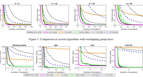
+xj j∈gk. For PA-SVRG and PA-SAGA, to explore the effect of accuracy on the convergence, we set the desired accuracy

= 10−4 _when _K _{= 5} _and_K _{= 10}_, _{= 10}−5 _when

(7)

0 20 40 60 80 100 Number of iterations 0

2 4 6 8

Objective value

K = 5

0 10 20 30 40 50 Number of iterations 0

2 4 6 8

Objective value

K = 10

0 10 20 30 40 50

Number of iterations 0

2 4 6 8

Objective value

K = 20

0 10 20 30 40

Number of iterations 0

2 4 6 8

Objective value

K = 50

APA-SVRG APA-SAGA PA-ASGD SVRG-ADMM PA-SVRG PA-SAGA

Figure 1: Comparison of several algorithms with overlapping group lasso.

0 5 10 15 20

Number of iterations 0.5

0.55 0.6 0.65

Objective value

German-numer

0 5 10 15 20

0.4 0.42 0.44 0.46 0.48

Objective value

a9a

0 5 10

0.2 0.25 0.3 0.35 0.4

Objective value

w7a

0 5 10

0.4 0.5 0.6

Objective value

cod-rna

APA-SVRG APA-SAGA PA-ASGD SVRG-ADMM PA-SVRG PA-SAGA

Figure 2: Comparison of several algorithms with graph-guided fused lasso.

Table 1: Summary of the datasets used in the graph-guided fused lasso experiments

Dataset #samples dimensionality λ

german-numer 1000 24 10−3

a9a 32561 123 10−4

w7a 24692 300 10−4

cod-rna 59353 8 10−4

the other hand, the adaptive stepzise strategy enables APA-SAGA and APA-SVRG to achieve a fast convergence rate while involving a simpler implementation as well as conver-gence analysis than SVRG-ADMM. Moreover, the perfor-mance of PA-ASGD is poor on all datasets.

Graph-Guided Logistic Regression

We proceed with the experiments on the graph-guided logis-tic regression (Kim and Xing 2009):

min

x∈Rd 1 n

n

X

i=1

log(1 + exp(−bix|ai))

+λ kxk2₊ X

{k1,k2}∈E

|xk1−xk2|

. (33)

Here,Eis the graph edge set, and we construct this graph by sparse inverse covariance selection (Friedman, Hastie, and Tibshirani 2008). For an edgekconnecting featurek1and

k2, proxγ_r_k(x)can be easily computed, and the value on its

j-th index is



 

 

xj−sign(xk1−xk2) min

γ,|xk₁−xk₂|

2 j=k1;

xj+sign(xk1−xk2) min

γ,|xk1−xk2|

2 j=k2;

xj otherwise.

We set the desired accuracy = 10−4 _{for PA-SVRG} and PA-SAGA. Figure 2 shows the experimental results. As can be seen, the performance of PA-ASGD is poor with-out the variance reduction technique. On the other side, the small stepsize limits the performance of SVRG and PA-SAGA. With a larger stepsize, APA-SVRG, APA-SAGA and SVRG-ADMM can quickly approach the optimal point. And the adaptive stepsize strategy enables the iterations of APA-SVRG and APA-SAGA to converge to the optimal point.

Conclusion

In this paper, we apply the adaptive stepsize strategy to the PA-based VR stochastic algorithms, and propose the corre-sponding APA-SVRG and APA-SAGA algorithms. By ini-tializing the stepsize with a relatively large value and adap-tively decreasing it, both proposed algorithms can achieve theO(nlog1

+m0

1

)iteration complexity. Moreover,

ex-periments on overlapping group lasso and graph-guided lo-gistic regression demonstrate the efficiency of the proposed methods.

Acknowledgement

(8)

References

Bauschke, H. H.; Goebel, R.; Lucet, Y.; and Wang, X. 2008. The proximal average: basic theory. SIAM Journal on Opti-mization19(2):766–785.

Bottou, L.; Curtis, F. E.; and Nocedal, J. 2016. Optimization methods for large-scale machine learning. arXiv preprint arXiv:1606.04838.

Boyd, S.; Parikh, N.; Chu, E.; Peleato, B.; Eckstein, J.; et al. 2011. Distributed optimization and statistical learning via the alternating direction method of multipliers.Foundations and TrendsR in Machine learning3(1):1–122.

Chang, C.-C., and Lin, C.-J. 2011. LIBSVM: A library for support vector machines. ACM Transactions on Intelligent Systems and Technology2:27:1–27:27. Software available at http://www.csie.ntu.edu.tw/∼_{cjlin/libsvm.}

Chen, X.; Lin, Q.; Kim, S.; Carbonell, J. G.; Xing, E. P.; et al. 2012. Smoothing proximal gradient method for general structured sparse regression. The Annals of Applied Statis-tics6(2):719–752.

Cheung, Y.-m., and Lou, J. 2017. Proximal average approx-imated incremental gradient descent for composite penalty regularized empirical risk minimization. Machine Learning

106(4):595–622.

Defazio, A.; Bach, F.; and Lacoste-Julien, S. 2014. Saga: A fast incremental gradient method with support for non-strongly convex composite objectives. InAdvances in Neu-ral Information Processing Systems, 1646–1654.

Defazio, A.; Domke, J.; et al. 2014. Finito: A faster, per-mutable incremental gradient method for big data problems. In International Conference on Machine Learning, 1125– 1133.

Friedman, J.; Hastie, T.; and Tibshirani, R. 2008. Sparse inverse covariance estimation with the graphical lasso. Bio-statistics9(3):432–441.

Hastie, T.; Tibshirani, R.; and Friedman, J. 2001. The Ele-ments of Statistical Learning. Springer Series in Statistics. New York, NY, USA: Springer New York Inc.

Jacob, L.; Obozinski, G.; and Vert, J.-P. 2009. Group lasso with overlap and graph lasso. In Proceedings of the 26th annual international conference on machine learning, 433– 440. ACM.

Johnson, R., and Zhang, T. 2013. Accelerating stochastic gradient descent using predictive variance reduction. In Ad-vances in neural information processing systems, 315–323. Kim, S., and Xing, E. P. 2009. Statistical estimation of cor-related genome associations to a quantitative trait network.

PLoS genetics5(8):e1000587.

Liu, J.; Wright, S. J.; R´e, C.; Bittorf, V.; and Sridhar, S. 2015. An asynchronous parallel stochastic coordinate de-scent algorithm.The Journal of Machine Learning Research

16(1):285–322.

Nesterov, Y. 2005. Smooth minimization of non-smooth functions. Mathematical programming103(1):127–152.

Nesterov, Y. 2013. Introductory lectures on convex

opti-mization: A basic course, volume 87. Springer Science & Business Media.

Nguyen, L. M.; Liu, J.; Scheinberg, K.; and Tak´aˇc, M. 2017. SARAH: A novel method for machine learning problems us-ing stochastic recursive gradient. In International Confer-ence on Machine Learning, volume 70, 2613–2621. PMLR. Ouyang, H., and Gray, A. 2012. Stochastic smoothing for nonsmooth minimizations: Accelerating sgd by exploiting structure. arXiv preprint arXiv:1205.4481.

Ouyang, H.; He, N.; Tran, L.; and Gray, A. 2013. Stochastic alternating direction method of multipliers. InInternational Conference on Machine Learning, 80–88.

Owen, A. B. 2013.Monte Carlo theory, methods and exam-ples.

Pedregosa, F., and Gidel, G. 2018. Adaptive three opera-tor splitting. In Dy, J., and Krause, A., eds.,International Conference on Machine Learning, 4085–4094.

Pedregosa, F.; Fatras, K.; and Casotto, M. 2018. Vari-ance reduced three operator splitting. arXiv preprint arXiv:1806.07294.

Qin, Z., and Goldfarb, D. 2012. Structured sparsity via alternating direction methods.Journal of Machine Learning Research13(May):1435–1468.

Robbins, H., and Monro, S. 1951. A stochastic approxima-tion method.The annals of mathematical statistics400–407. Schmidt, M.; Le Roux, N.; and Bach, F. 2017. Minimizing finite sums with the stochastic average gradient. Mathemat-ical Programming162(1-2):83–112.

Shen, L.; Liu, W.; Huang, J.; Jiang, Y.-G.; and Ma, S. 2017. Adaptive proximal average approximation for composite convex minimization. InAAAI, 2513–2519.

Singer, Y., and Duchi, J. C. 2009. Efficient learning using forward-backward splitting. In Advances in Neural Infor-mation Processing Systems 22, 495–503.

Suzuki, T. 2014. Stochastic dual coordinate ascent with alternating direction method of multipliers. InInternational Conference on Machine Learning, 736–744.

Xiao, L., and Zhang, T. 2014. A proximal stochastic gradient method with progressive variance reduction. SIAM Journal on Optimization24(4):2057–2075.

Yu, Y.; Zheng, X.; Marchetti-Bowick, M.; and Xing, E. 2015. Minimizing nonconvex non-separable functions. In

Artificial Intelligence and Statistics, 1107–1115.

Yu, Y.-L. 2013. Better approximation and faster algorithm using the proximal average. InAdvances in neural informa-tion processing systems, 458–466.

Zhao, P.; Rocha, G.; and Yu, B. 2009. The composite ab-solute penalties family for grouped and hierarchical variable selection.The Annals of Statistics3468–3497.

Zheng, S., and Kwok, J. T. 2016. Fast-and-light stochastic admm. InIJCAI, 2407–2613.