Statistical multipole formulations for shielding problems

(1)

Adv. Radio Sci., 10, 233–238, 2012 www.adv-radio-sci.net/10/233/2012/ doi:10.5194/ars-10-233-2012

Advances in

Radio Science

Statistical multipole formulations for shielding problems

K. K¨orber and L. Klinkenbusch

Christian-Albrechts-Universit¨at zu Kiel, Computational Electromagnetics Group, Kaiserstr. 2, 24143 Kiel, Germany Correspondence to: K. K¨orber ([email protected])

Abstract. A multipole-based method is presented for mod-elling an electromagnetic field with small statistical varia-tions inside an arbitrary enclosure. The accurate computa-tion of the statistics of the field components from the statisti-cal moments of the multipole amplitudes is demonstrated for two- and three-dimensional examples. To obtain the statistics of quantities which depend non-linearly on the field compo-nents, higher-order statistical moments of the latter are re-quired.

1 Introduction

Recent research in the field of statistical electromagnetics in general and statistical EMC in particular seems to focus on extremely non-deterministic fields as observed in a reverber-ation chamber. Much progress has been achieved in this area over the last decades, leading to very general statistical power distributions largely independent of the chamber geometry (Holland, 1999). Relatively little work has been done on the topic of small statistical variations of an otherwise known electromagnetic field. A related example relevant to EMC has been presented in (Ajayi et al., 2008).

In this paper we discuss the case of small statistical vari-ations in various parameters of a shielding problem, e.g. the angle of incidence of a plane wave impinging on a shield. The varying parameters are given by the first few statisti-cal moments of their distributions. From these the statististatisti-cal moments of the amplitudes of a spherical-multipole expan-sion are derived. The statistics of the multipole amplitudes then characterizes the statistical properties of the electromag-netic field not only in a single point but in a spherical re-gion around the arbitrarily chosen center of the expansion. In practice, this spherical region can be part of the enclosed volume of any shielding structure. For non-canonical prob-lems, where the calculation of the multipole amplitudes can-not be achieved analytically, data from numerical simulations

or measurements are needed to estimate the statistical mo-ments of the multipole amplitudes.

2 Multipole expansion

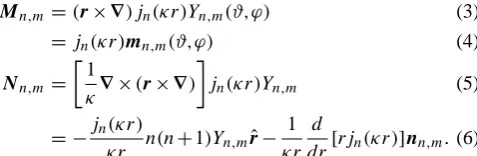
Consider an arbitrary shielding structure as depicted in Fig. 1.

The electromagnetic field in any linear, homogeneous, and source-free spherical sub-domain of the enclosure can be ex-panded by means of a spherical-multipole expansion:

E =

∞ P

n=1 n

P

m=−n

An,mNn,m+Z_j ∞ P

n=1 n

P

m=−n

Bn,mMn,m (1)

H =j Z

∞ P

n=1 n

P

m=−n

An,mMn,m+ ∞ P

n=1 n

P

m=−n

Bn,mNn,m. (2) The coefficientsAn,mandBn,m are referred to as the elec-tric and magnetic multipole amplitudes, respectively, Z= √

µ/ε is the wave impedance in the spherical sub-domain andMn,m,Nn,mrepresent the spherical-multipole functions defined by

Mn,m=(r×∇)jn(κr)Yn,m(ϑ,ϕ) (3)

=jn(κr)mn,m(ϑ,ϕ) (4)

Nn,m=

₁

κ∇×(r×∇)

jn(κr)Yn,m (5)

= −jn(κr)

κr n(n+1)Yn,mrˆ− 1 κr

d

dr[rjn(κr)]nn,m.(6) Here, jn(κr) denote spherical Bessel functions of the 1st kind, rˆ is the radial unit vector, and the vector wave func-tions are found as:

mn,m(ϑ,ϕ)= − 1 sinϑ

∂Yn,m ∂ϕ

ˆ

ϑ+∂Yn,m

∂ϑ ϕˆ (7)

nn,m(ϑ,ϕ)= + ∂Yn,m

∂ϑ ˆ

ϑ+ 1

sinϑ ∂Yn,m

∂ϕ ϕˆ. (8)

(2)

234 K. K¨orber and L. Klinkenbusch: Statistical multipole formulations for shielding problems

Manuscript prepared for Adv. Radio Sci. with version 4.2 of the LA_{TEX class copernicus.cls.} Date: 20 February 2012

Statistical Multipole Formulations for Shielding Problems

K. K¨orber and L. Klinkenbusch

Christian-Albrechts-Universit¨at zu Kiel, Computational Electromagnetics Group, Kaiserstr. 2, 24143 Kiel, Germany

Abstract. A multipole-based method is presented for mod-elling an electromagnetic field with small statistical varia-tions inside an arbitrary enclosure. The accurate computa-tion of the statistics of the field components from the statisti-cal moments of the multipole amplitudes is demonstrated for 5

two- and three-dimensional examples. To obtain the statistics of quantities which depend non-linearly on the field compo-nents, higher-order statistical moments of the latter are re-quired.

10

1 Introduction

Recent research in the field of statistical electromagnetics in general and statistical EMC in particular seems to focus on extremely non-deterministic fields as observed in a reverber-ation chamber. Much progress has been achieved in this area 15

over the last decades, leading to very general statistical power distributions largely independent of the chamber geometry (Holland, 1999). Relatively little work has been done on the topic of small statistical variations of an otherwise known electromagnetic field. A related example relevant to EMC 20

has been presented in (Ajayi et al., 2008).

In this paper we discuss the case of small statistical vari-ations in various parameters of a shielding problem, e.g. the angle of incidence of a plane wave impinging on a shield. The varying parameters are given by the first few statisti-25

cal moments of their distributions. From these the statistical moments of the amplitudes of a spherical-multipole expan-sion are derived. The statistics of the multipole amplitudes then characterizes the statistical properties of the electromag-netic field not only in a single point but in a spherical re-30

gion around the arbitrarily chosen center of the expansion. In practice, this spherical region can be part of the enclosed

Correspondence to:Kai K¨orber ([email protected])

Fig. 1.Spherical domain inside an arbitrary shielding enclosure.

volume of any shielding structure. For non-canonical prob-lems, where the calculation of the multipole amplitudes can-not be achieved analytically, data from numerical simulations 35

or measurements are needed to estimate the statistical mo-ments of the multipole amplitudes.

2 Multipole expansion

Consider an arbitrary shielding structure as depicted in Fig-ure 1. The electromagnetic field in any linear, homogeneous, 40

and source-free spherical sub-domain of the enclosure can be expanded by means of a spherical-multipole expansion:

E = ∞

P

n=1 n

P

m=−n

An,mNn,m+Z_j

∞

P

n=1 n

P

m=−n

Bn,mMn,m (1)

H=_Zj ∞

P

n=1 n

P

m=−n

An,mMn,m+

∞

P

n=1 n

P

m=−n

Bn,mNn,m. (2)

The coefficientsAn,mandBn,mare referred to as the

elec-45

tric and magnetic multipole amplitudes, respectively, Z=

p

µ/ε is the wave impedance in the spherical sub-domain and Mn,m, Nn,m represent the spherical-multipole

func-Fig. 1. Spherical domain inside an arbitrary shielding enclosure.

The normalized surface-spherical harmonics are given by

Yn,m(ϑ,ϕ)=

s

2n+1 4π

(n−m)! (n+m)!P

m

n (cosϑ )ej mϕ (9) withP_nmbeing associated Legendre functions of the 1st kind. For two-dimensional problems, a cylindrical-multipole ex-pansion in plane-polar coordinates(R,ϕ)consisting of ordi-nary Bessel-functionsJn inRand harmonic functions inϕ can be applied. For the TMz-case this takes the following form (Klinkenbusch, 2005):

Ez(R,ϕ)= ∞ X

n=−∞

anJn(κR)ej nϕ (10)

HR(R,ϕ)= j Z

1 κR

∂

∂ϕEz(R,ϕ) (11)

Hϕ(R,ϕ)= −j Z

1 κ

∂

∂REz(R,ϕ). (12)

In any of the described cases, the complete information about the field is contained in the complex-valued multipole ampli-tudes (An,m, Bn,m; an). Consequently, the statistics of an electromagnetic field inside the enclosure can be reduced to the statistics of the corresponding multipole amplitudes.

3 Statistical formulation

To describe a statistically varying electromagnetic field we assume its multipole amplitudes to be random variables. For a spherical-multipole expansion truncated atn=nmaxthere arenmax(nmax+2)index pairs(n,m). For each(n,m)four real random variables need to be considered:

Re{An,m},Im{An,m},Re{Bn,m},Im{Bn,m}. (13) We introduce the multipole-amplitude random vectorV con-sisting of all multipole amplitudes considered. It thus has the lengthimax=4nmax(nmax+2).

This random vector V will be described by its first few moments, particularly by its expectation valueηV and its co-variance matrixCV (Papoulis, 2008).

3.1 Computation of field statistics

Once the multipole-amplitude random vector V is known in terms of its statistical moments, the field statistics at any points in the domain, where the multipole expansion is valid, can be easily calculated. To this end, we first construct a new field-component random vectorW consisting of all real and imaginary parts of all field components at any desired point in the domain. Because of the linearity of the multi-pole expansion (Eqs. 1–2) the field-component random vec-torW=g(V)depends linearly on the multipole-amplitude random vectorV, hence the statistical moments ofW are easily obtained from the statistical moments ofV. For the first two moments (expectation value and covariance matrix) this leads to:

ηWk =gk(ηV) (14)

CW_k,Wl = X

i

X

j CV_i,Vj

∂gk ∂vi

_ηV

∂gl ∂vj

ηV

. (15)

Note that for this linear relation n-th order moments ofW only depend onn-th order moments ofV.

This means that the complete field statistics of the whole domain, where the multipole expansion is valid, is contained in the moments of V. Usually, the first two moments are sufficient, for arbitrary accuracy higher order moments like skew, curtosis, etc. – as well as their correlations – may have to be considered.

3.2 Compactness of description

The proposed approach of a statistical multipole expansion is a very efficient and systematic way of modelling an elec-tromagnetic field with small variations.

As an example consider the field in a cubic volume of edge length 1.6 m centered around the point of origin at a frequency of 750 MHz (as used in the first examples of Sect. 4). In this case the multipole expansion can be trun-cated atnmax≈20 for sufficient accuracy, which leads to a random vector of lengthimax≈1760. On the other hand, to describe the statistics of the field components at each point in space, at least six real random variables would be required per position, i.e. the quadrature components of either the electric or the magnetic field. At a reasonable spatial reso-lution of at least ten points per wavelength this amounts to a random vector of lengthimax≈384000.

The impact of this difference is even larger when consider-ing that, while the length of the vector of expectation values ηisimax, the number of entries in the correlation matrixCis i2_max.

A similar result is obtained for a cylindrical expansion of a square domain of 1.6 m×1.6 m. At 750 MHz the statis-tical multipole expansion leads toimax≈194, the pointwise description of the field components’ statistics toimax≈3200.

(3)

K. K¨orber and L. Klinkenbusch: Statistical multipole formulations for shielding problems 235

3.3 Sources of statistical variations

To test this new approach we start with a simple example, that is, the electromagnetic field of a homogeneous plane wave where we add a small statistical variation using a single nor-mally distributed real random variableU.

The spherical multipole expansion’s (Eqs. 1–2) amplitudes of a plane wave are known (Klinkenbusch, 1996):

An,m=E04πjn+1 (−1) m n(n+1)

h

nn,−m(ϑ,ϕ)· ˆξ i

ϑ0,ϕ0

(16) Bn,m=

E0 Z 4πj

n+1 (−1)m n(n+1)

h

mn,−m(ϑ,ϕ)· ˆξ

i

ϑ0,ϕ0

. (17) Here,E0andξˆ are amplitude and polarization of the plane wave, while(ϑ0,ϕ0)denote its angle of incidence.

For the two-dimensional TMz-case, the multipole ampli-tudes of a plane wave of amplitudeE0and angle of incidence ϕ0are (Klinkenbusch, 2005):

an=E0jne−j nϕ0_. ₍₁₈₎

First we will vary the phase. This can be easily done by mul-tiplying the known amplitudes by a phase factor containing the random variableUas follows:

A0_n,m=An,mej U (19)

B_n,m0 =Bn,mej U (20)

a_n0 =anej U. (21)

A practically more interesting case is the variation of the an-gle of incidence. This will be realized by replacing the anan-gle ϕ0 in Eqs. (16–18) with a random variable U as described above.

With these relations between the given random variableU and the multipole-amplitude random vectorV =g(U ), the moments ofV can be calculated. Since U is a single real random variable (not a random vector), the expectation val-ues and covariance matrix ofV are as follows:

ηV_i =gi(ηU)+ ∞ X

n=2 µn(U )

n! g (n)

i (ηU) (22)

CVi,Vj = ∞ X

n=2 µn(U )

n! n−1

X

k=1

n k

g(k)_i (ηU)g(n −k) j (ηU)

!

(23)

− ∞ X

n=4 n−2

X

k=2

µk(U )µn−k(U ) k!(n−k)! g

(k) i (ηU)g(n

−k) j (ηU)

!

.

Hereµn(U )denotes then-th central moment ofU andg(k)_i is thek-th derivative ofgi with respect to its argument.

In this paper we chooseUto be normally distributed with zero mean, hence all even moments ofUare known in terms of its standard deviationσU (Abramowitz, 1972) and all odd moments are zero (see Table 1). For the following calcula-tions the moments ofU are considered up to and including eighth order.

Table 1. Central moments of a normally distributed random vari-able (Abramowitz, 1972).

n 1 2 3 4 5 6 7 8 . . .

µn 0 σ2 0 3σ4 0 15σ6 0 105σ8 . . .

K. K¨orber, L. Klinkenbusch: Statistical Multipole Formulations for Shielding Problems 3

3.3 Sources of statistical variations

To test this new approach we start with a simple example, that is, the electromagnetic field of a homogeneous plane wave where we add a small statistical variation using a single nor-mally distributed real random variableU.

140

The spherical multipole expansion’s (Eqs. (1-2)) ampli-tudes of a plane wave are known (Klinkenbusch, 1996):

An,m=E04πjn+1

(−1)m

n(n+ 1)

h

nn,−m(ϑ,ϕ)·ˆξ

i

ϑ0,ϕ0

(16)

Bn,m=

E0

Z 4πj

n+1 (−1)

m

n(n+ 1)

h

mn,−m(ϑ,ϕ)·ˆξ

i

ϑ0,ϕ0

. (17)

Here,E0andˆξare amplitude and polarization of the plane 145

wave, while(ϑ0,ϕ0)denote its angle of incidence.

For the two-dimensional TMz-case, the multipole

ampli-tudes of a plane wave of amplitudeE0and angle of incidence

ϕ0are (Klinkenbusch, 2005):

an=E0jne−jnϕ0. (18)

150

First we will vary the phase. This can be easily done by mul-tiplying the known amplitudes by a phase factor containing the random variableUas follows:

A0_n,m=An,mejU (19)

B_n,m0 =Bn,mejU (20)

155

a0_n=anejU. (21)

A practically more interesting case is the variation of the an-gle of incidence. This will be realized by replacing the anan-gle ϕ0 in Eqs. (16-18) with a random variableU as described

above. 160

With these relations between the given random variableU and the multipole-amplitude random vectorV =g(U), the moments ofV can be calculated. SinceU is a single real random variable (not a random vector), the expectation val-ues and covariance matrix ofV are as follows:

165

ηVi =gi(ηU) +

∞

X

n=2

µn(U)

n! g

(n)

i (ηU) (22)

CVi,Vj =

∞

X

n=2

µn(U)

n! n−1

X

k=1

n k

g_i(k)(ηU)g

(n−k)

j (ηU)

!

(23)

− ∞

X

n=4

n−2

X

k=2

µk(U)µn−k(U)

k!(n−k)! g

(k)

i (ηU)g

(n−k)

j (ηU)

!

.

Hereµn(U)denotes then-th central moment ofU andg

(k)

i

is thek-th derivative ofgiwith respect to its argument.

170

In this paper we chooseUto be normally distributed with zero mean, hence all even moments ofU are known in terms of its standard deviationσU (Abramowitz, 1972) and all odd

moments are zero (see Table 1). For the following calcula-tions the moments ofU are considered up to and including 175

eighth order.

Table 1. Central moments of a normally distributed random vari-able (Abramowitz, 1972)

n 1 2 3 4 5 6 7 8 . . .

µn 0 σ2 0 3σ4 0 15σ6 0 105σ8 . . .

++++

Fig. 2. Expectation valueη(upper plot) and standard deviationσ

(central plot) ofRe{Ez}according to statistical multipole calcula-tion (SM) and Monte Carlo simulacalcula-tion (MC) for a plane wave with varying phase (σψ= 20◦). The lower plot displays the differences between statistical multipole calculation and Monte Carlo simula-tion.

4 Results

4.1 Plane wave

Figure 2 shows the results for a plane wave with a vary-ing phase ψ of standard deviation σψ= 20◦ at frequency

180

f= 750MHz. The upper diagram represents the expectation valueη of the real part ofEz and includes the

correspond-ing standard deviationσSM. The central diagram shows the

standard deviationσSM alone. Both are calculated by the

aforementioned method and - for reference - by a Monte-185

Carlo simulation (IndexM C). The absolute differences

be-tween the spherical-multipole calculations are also shown in the lower diagram.

As expected, for a varying phase the standard deviation is largest at the inflection points of the sine curve and mini-190

mal at the extreme values. The accordance with Monte Carlo simulations is excellent.

Figure 3 shows the results for a plane wave along the main axis, where the angle of incidenceϕ0is varied according to

a standard deviation ofσϕ0= 5 ◦_, 195

Again, the influence of the angle of incidence on the field is largest at the sine curve’s inflexion points and minimal at Fig. 2. Expectation value η(upper plot) and standard deviation σ (central plot) of Re{Ez}according to statistical multipole cal-culation (SM) and Monte Carlo simulation (MC) for a plane wave with varying phase (σψ=20◦). The lower plot displays the dif-ferences between statistical multipole calculation and Monte Carlo simulation.

4 Results

4.1 Plane wave

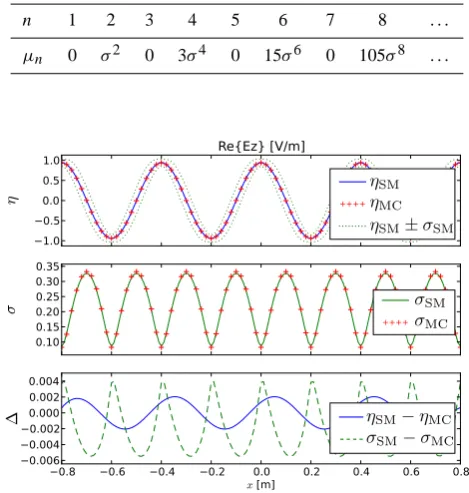
Figure 2 shows the results for a plane wave with a vary-ing phase ψ of standard deviation σψ=20◦ at frequency f=750 MHz. The upper diagram represents the expectation valueηof the real part ofEzand includes the corresponding standard deviationσSM. The central diagram shows the stan-dard deviationσSM alone. Both are calculated by the afore-mentioned method and – for reference – by a Monte-Carlo simulation (IndexMC). The absolute differences between the spherical-multipole calculations are also shown in the lower diagram.

As expected, for a varying phase the standard deviation is largest at the inflection points of the sine curve and mini-mal at the extreme values. The accordance with Monte Carlo simulations is excellent.

Figure 3 shows the results for a plane wave along the main axis, where the angle of incidenceϕ0is varied according to a standard deviation ofσϕ0=5

◦_.

(4)

4 K. K¨orber, L. Klinkenbusch: Statistical Multipole Formulations for Shielding Problems

Fig. 3. Expectation value and standard deviation ofRe{Ez} ac-cording to statistical multipole calculation and Monte Carlo simu-lation for a plane wave with varying incident angle (σϕ0= 5

◦ ). For a legend see Fig. 2.

the extreme values, and the agreement with the Monte Carlo simulations is excellent.

4.2 Slitted cylinder 200

To test our approach with a simple shielding geometry we have used the geometry shown in Fig. 4 representing a thin slitted PEC-cylinder with radiusRS and aperture angleβ,

illuminated by a plane wave polarized in thez-direction and incident atϕ0. For the deterministic solution of this problem 205

see (Klinkenbusch, 2005).

Figure 5 shows the expectation value of the imaginary part ofEz in thex-y-plane. The shape of the cylinder with

R0= 0.5m and β= 40◦ is displayed as a black line, the

angle of incidence is varying around its expectation value 210

PEC incident field

Fig. 4.Geometry of the slitted PEC cylinder in thex-y-plane

Fig. 5. Expectation value ofIm{Ez}according to statistical mul-tipole calculation for a slitted cylinder illuminated by a plane wave with varying angle of incidence (σϕ0= 5

◦ )

ηϕ0= 135

◦_{with standard deviation}_σ

ϕ0= 5

◦_{. The frequency}

of the incident field is750MHz.

Figure 6 shows in detail the corresponding expectation val-ues, standard deviations and their comparison to Monte Carlo simulations (as in Figs. 2-3) along thex-axis (the dashed line 215

in Fig. 5).

Compared to the previous examples the field structure is much more complex and the standard deviation reaches much larger values. However the multipole expansion again

Fig. 6. Expectation value and standard deviation ofIm{Ez} ac-cording to statistical multipole calculation and Monte Carlo simula-tion for a slitted cylinder illuminated by a plane wave with varying angle of incidence (σϕ0= 5

◦

). For a legend see Fig. 2. Fig. 3. Expectation value and standard deviation of Re{Ez}

accord-ing to statistical multipole calculation and Monte Carlo simulation for a plane wave with varying incident angle (σϕ0=5

◦_{). For a}

leg-end see Fig. 2.

Again, the influence of the angle of incidence on the field is largest at the sine curve’s inflexion points and minimal at the extreme values, and the agreement with the Monte Carlo simulations is excellent.

4.2 Slitted cylinder

To test our approach with a simple shielding geometry we have used the geometry shown in Fig. 4 representing a thin slitted PEC-cylinder with radius RS and aperture angleβ, illuminated by a plane wave polarized in thez-direction and incident atϕ0. For the deterministic solution of this problem see (Klinkenbusch, 2005).

Figure 5 shows the expectation value of the imaginary part ofEz in thex-y-plane. The shape of the cylinder with R0=0.5 m and β=40◦ is displayed as a black line, the angle of incidence is varying around its expectation value ηϕ0=135

◦_{with standard deviation}_σ ϕ0=5

◦_{. The frequency} of the incident field is 750 MHz.

Figure 6 shows in detail the corresponding expectation val-ues, standard deviations and their comparison to Monte Carlo simulations (as in Figs. 2–3) along thex-axis (the dashed line in Fig. 5).

Compared to the previous examples the field structure is much more complex and the standard deviation reaches much larger values. However the multipole expansion again shows excellent correspondence with the Monte Carlo simu-lation particularly inside the shield.

◦_{). For}

a legend see Fig. 2.

To test our approach with a simple shielding geometry we have used the geometry shown in Fig. 4 representing a thin slitted PEC-cylinder with radius RS and aperture angleβ,

illuminated by a plane wave polarized in thez-direction and incident atϕ0. For the deterministic solution of this problem

205

PEC incident field

◦₎

ηϕ0= 135◦with standard deviationσϕ0= 5◦. The frequency

in Fig. 5).

◦_{). For a legend see Fig. 2.} Fig. 4. Geometry of the slitted PEC cylinder in thex-y-plane.

◦_{). For}

a legend see Fig. 2.

illuminated by a plane wave polarized in thez-direction and incident atϕ0. For the deterministic solution of this problem

205

PEC incident field

◦₎

ηϕ0= 135◦with standard deviationσϕ0= 5◦. The frequency

in Fig. 5).

◦_{). For a legend see Fig. 2.}

Fig. 5. Expectation value of Im{Ez}according to statistical multi-pole calculation for a slitted cylinder illuminated by a plane wave with varying angle of incidence (σϕ0=5

◦_).

4.3 Shielding effectiveness

The electromagnetic shielding effectiveness has been shown to be an adequate quantity for the characterization of a shield for the high-frequency case (Klinkenbusch, 1996). It is de-fined as:

SEem=10log10 2 |Esh_|2

|Eun_|2+

|Hsh_|2

|Hun_|2

. (24)

The quantities marked withshare for the shielded case, while those marked un are for the unshielded case, i.e. the case where no shield is present at all. For the example in Sect. 4.2 the corresponding unshielded fields |Eun| and |Hun| are those of an undisturbed plane wave and thus are constant. The fields for the shielded case are those of Sect. 4.2 de-scribed by the random vectorW. The random variable for

(5)

K. K¨orber and L. Klinkenbusch: Statistical multipole formulations for shielding problems 237

◦ ). For a legend see Fig. 2.

illuminated by a plane wave polarized in thez-direction and incident atϕ0. For the deterministic solution of this problem 205

PEC incident field

◦₎

ηϕ0= 135

◦_{with standard deviation}_σ

ϕ0= 5

◦_{. The frequency}

in Fig. 5).

◦_{). For a legend see Fig. 2.}

Fig. 6. Expectation value and standard deviation of Im{Ez} accord-ing to statistical multipole calculation and Monte Carlo simulation for a slitted cylinder illuminated by a plane wave with varying angle of incidence (σϕ0=5

◦

). For a legend see Fig. 2.

Fig. 7. Expectation value ofSEemaccording to statistical multi-pole calculation for a slitted cylinder illuminated by a plane wave with varying angle of incidence (σϕ0= 5

◦ )

shows excellent correspondence with the Monte Carlo simu-220

lation particularly inside the shield.

4.3 Shielding effectiveness

The electromagnetic shielding effectiveness has been shown to be an adequate quantity for the characterization of a shield for the high-frequency case (Klinkenbusch, 1996). It is de-225

fined as:

SEem= 10log10

2

|Esh_|2 |Eun_|2+

|Hsh_|2 |Hun_|2

. (24)

The quantities marked withshare for the shielded case, while those markedun are for the unshielded case, i.e. the case where no shield is present at all. For the example in Sect. 4.2 230

the corresponding unshielded fields |Eun_| _and _|_Hun_| _are

those of an undisturbed plane wave and thus are constant. The fields for the shielded case are those of Sect. 4.2 de-scribed by the random vectorW. The random vector of the shielding effectiveness values will be calledX. To compare 235

the results with those ones of the simple cases described be-fore we consider the expectation value and the standard de-viation of the shielding effectiveness. These are calculated from the relations

ηX =g(ηW) +

X

i

X

j

CWi,Wj

2

∂2_g

∂wi∂wj

ηW

+... (25) 240

σX2 =

X

i

X

j

CWi,Wj ∂g ∂wi ηW ∂g ∂wj ηW

+... (26)

Figure 7 shows the expectation value ofSEemin thex-y

-plane. Figure 8 shows in detail the corresponding expectation

Fig. 8.Expectation value and standard deviation ofSEem accord-ing to statistical multipole calculation and Monte Carlo simulation for a slitted cylinder illuminated by a plane wave with varying angle of incidence (σϕ0= 5

◦

values, standard deviations and their comparison to Monte Carlo simulations along thex-axis. All parameters are iden-245

tical to those in Figs. 5-6.

While the error of the expectation value is still quite small, the standard deviation derived from the multipole evaluation differs significantly from the Monte Carlo simulation. This can be explained by Eqs. (25-26). The moments ofX de-250

pend on all moments ofW, but unlike Eqs. (22-23), where all moments of the normally distributed random variableU were known, in this case only the expectation values and co-variance matrix ofW have been taken into account for this calculation. Obviously that is not sufficient for a non-linear 255

relation like Eq. (24).

This clearly shows that for the statistics of quantities that depend in a non-linear fashion on the field components, also higher order moments of the multipole amplitudes have to be taken into account.

260

5 Conclusions

For calculating the statistical moments of the electromag-netic field in case of small variations of various parame-ters, the statistical-multipole method yields similar results as Monte Carlo simulations with the advantage that the number 265

of quantities to represent the field and its statistics is greatly reduced. However, modeling the multipole-amplitude ran-dom vector in terms of only first and second order statistical moments has been shown to be insufficient for the compu-tation of the moments of quantities, which non-linearly de-270

pend on the multipole amplitudes like the electromagnetic shielding effectiveness. In such cases higher-order statisti-Fig. 7. Expectation value of SEemaccording to statistical multipole

calculation for a slitted cylinder illuminated by a plane wave with varying angle of incidence (σϕ0=5

◦_).

the shielding effectiveness will be calledX. To compare the results with those ones of the simple cases described before we consider the expectation value and the standard deviation of the shielding effectiveness. These are calculated from the relations

ηX=g(ηW)+

X

i

X

j

CW_i,Wj 2

∂2g ∂wi∂wj ηW

+... (25)

Fig. 7. Expectation value ofSEemaccording to statistical multi-pole calculation for a slitted cylinder illuminated by a plane wave with varying angle of incidence (σϕ0= 5

◦

)

shows excellent correspondence with the Monte Carlo simu-220

lation particularly inside the shield.

4.3 Shielding effectiveness

The electromagnetic shielding effectiveness has been shown to be an adequate quantity for the characterization of a shield for the high-frequency case (Klinkenbusch, 1996). It is de-225

fined as:

SEem= 10log10

2

|Esh_|2 |Eun_|2+

|Hsh_|2 |Hun_|2

. (24)

The quantities marked withsh_{are for the shielded case, while}

those markedun are for the unshielded case, i.e. the case where no shield is present at all. For the example in Sect. 4.2 230

the corresponding unshielded fields |Eun_| _and _|_Hun_| _are

those of an undisturbed plane wave and thus are constant. The fields for the shielded case are those of Sect. 4.2 de-scribed by the random vectorW. The random vector of the shielding effectiveness values will be calledX. To compare 235

the results with those ones of the simple cases described be-fore we consider the expectation value and the standard de-viation of the shielding effectiveness. These are calculated from the relations

ηX=g(ηW) +

X

i

X

j

CWi,Wj

2

∂2g ∂wi∂wj

ηW

+... (25) 240

σ_X2 =X i

X

j

CWi,Wj ∂g ∂wi ηW ∂g ∂wj ηW

+... (26)

Figure 7 shows the expectation value ofSEem in thex-y

-plane. Figure 8 shows in detail the corresponding expectation

Fig. 8.Expectation value and standard deviation ofSEem accord-ing to statistical multipole calculation and Monte Carlo simulation for a slitted cylinder illuminated by a plane wave with varying angle of incidence (σϕ0= 5

◦

values, standard deviations and their comparison to Monte Carlo simulations along thex-axis. All parameters are iden-245

tical to those in Figs. 5-6.

While the error of the expectation value is still quite small, the standard deviation derived from the multipole evaluation differs significantly from the Monte Carlo simulation. This can be explained by Eqs. (25-26). The moments ofX de-250

pend on all moments ofW, but unlike Eqs. (22-23), where all moments of the normally distributed random variableU were known, in this case only the expectation values and co-variance matrix ofW have been taken into account for this calculation. Obviously that is not sufficient for a non-linear 255

relation like Eq. (24).

260

5 Conclusions

For calculating the statistical moments of the electromag-netic field in case of small variations of various parame-ters, the statistical-multipole method yields similar results as Monte Carlo simulations with the advantage that the number 265

of quantities to represent the field and its statistics is greatly reduced. However, modeling the multipole-amplitude ran-dom vector in terms of only first and second order statistical moments has been shown to be insufficient for the compu-tation of the moments of quantities, which non-linearly de-270

pend on the multipole amplitudes like the electromagnetic shielding effectiveness. In such cases higher-order statisti-Fig. 8. Expectation value and standard deviation of SEemaccording to statistical multipole calculation and Monte Carlo simulation for a slitted cylinder illuminated by a plane wave with varying angle of incidence (σϕ0=5

◦

σ_X2 =X i

X

j

CW_i,Wj ∂g ∂wi ηW ∂g ∂wj ηW

+... (26)

Figure 7 shows the expectation value of SEem in the x –y-plane. Figure 8 shows in detail the corresponding expectation values, standard deviations and their comparison to Monte Carlo simulations along thex-axis. All parameters are iden-tical to those in Figs. 5–6.

While the error of the expectation value is still quite small, the standard deviation derived from the multipole evaluation differs significantly from the Monte Carlo simulation. This can be explained by Eqs. (25–26). The moments ofX de-pend on all moments ofW, but unlike Eqs. (22–23), where all moments of the normally distributed random variableU were known, in this case only the expectation values and co-variance matrix ofW have been taken into account for this calculation. Obviously that is not sufficient for a non-linear relation like Eq. (24).

5 Conclusions

For calculating the statistical moments of the electromag-netic field in case of small variations of various parame-ters, the statistical-multipole method yields similar results as Monte Carlo simulations with the advantage that the number of quantities to represent the field and its statis-tics is greatly reduced. However, modeling the

(6)

amplitude random vector in terms of only first and second order statistical moments has been shown to be insufficient for the computation of the moments of quantities, which non-linearly depend on the multipole amplitudes like the elec-tromagnetic shielding effectiveness. In such cases higher-order statistical moments of the statistical multipole expan-sion have to be considered. However, the basic advantage of representing the field by a minimum number of parameters is still preserved.

Further research includes the application of the method to more general, that is, non-canonical shielding problems, and to characterize the shielding effect by the first few terms of the corresponding multipole expansion and its statistical mo-ments.

References

Ajayi, A., Ingrey, P., Sewell, P., and Christopoulos, C.: Direct Com-putation of Statistical Variations in Electromagnetic Problems, IEEE T. Electromagn. C., 50, 325–332, 2008.

Abramowitz, M. and Stegun, I. A. (eds.): Handbook of Mathemati-cal Functions with Formulas, Graphs, and MathematiMathemati-cal Tables, Applied mathematics series 55. US Government Printing Office, Washington, DC, USA, Tenth Printing, with corrections edition, 1972.

Holland, R. and St. John, R.: Statistical Electromagnetics, Taylor and Francis, 1999.

Klinkenbusch, L.: Theorie der sph¨arischen Absorberkammer und des mehrschaligen Kugelschirmes, Habilitationsschrift, Ruhr-Universit¨at Bochum, 1996.

Klinkenbusch, L.: On the shielding effectiveness of enclosures, IEEE T. Electromagn. C., 47, 589–601, 2005.

Papoulis, A. and Pillai, S. U.: Probability, random variables, and stochastic processes, McGraw-Hill series in electrical and com-puter engineering, McGraw-Hill, Boston, USA, 4th edn., 2008.