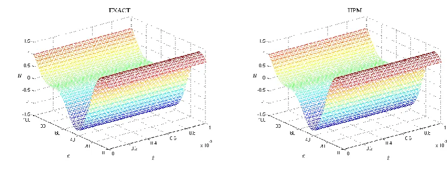
The Homotopy Perturbation Method for Solving the Kuramoto – Sivashinsky Equation

Encouraging early signals of clinical activity were also observed in other malignancies including non-small cell lung cancer (NSCLC), glioblastoma (GBM),

In the soil, heterogeneously distributed microbe communities together with dependent rhizobia and different plant growth promoting rhizobacteria perform a dynamic

Given the limited amount of undeveloped land in the City of Rutland, and the need to conserve some areas for open space and recreation, the primary potential for development is in

Other reasons given include the provision of education on the effects of drugs, religious beliefs, observation of the effects of drug abuse on past users, personal discipline

Aim is to understand the phenomenon of the training of teachers of physical education through a survey on the levels of education and measurement of the teachers’

Effective practices and models for older adults with SMI need to consider how services are delivered (e.g., mobile units, transporta- tion support, integrated health care

´ Sniatycki, Differential Geometry of Singular Spaces and Reduction of Symmetry, Cambridge University Press, Cambridge, 2013.

So, in patients presented with generalized tonic-clonic seizure also the possibility of ring enhancing lesion should be considered.. This correlates with the Sotelo