Abigo et al. World Journal of Engineering Research and Technology
APPLICATION OF ARTIFICIAL NEURAL NETWORK IN
OPTIMIZATION OF SOAP PRODUCTION
Izabo Abigo*1, Isaac E. Okwu2 and Barinyima Nkoi3
1
Mechanical Engineering Department/Rivers State University, Port Harcourt, Nigeria. 2
Mechanical Engineering Department/Rivers State University, Port Harcourt, Nigeria.
3
Mechanical Engineering Department/Rivers State University, Port Harcourt, Nigeria.
Article Received on 07/11/2018 Article Revised on 28/11/2018 Article Accepted on 19/12/2018
ABSTRACT
This project was aimed at optimizing soap production profit using
Neural Network programming. In this project a Neural Network was
trained using a data set of solved linear programming problems. The
objective function used in this training had two (2) variables and three
(3) constraints equations. This trained Neural Network was used to
optimize soap production profit for two different kinds of soap; bathing and laundry soaps.
The Neural Network structure consisted of eleven (11) inputs and 3 outputs with a neural
structure of 2 hidden layers and 50 neurons. The training algorithm used was feed-forward
back propagation with a Bayesian Regularization error. The Neural Network results when
compared with traditional simplex method of optimization, proved to be 98% accurate. The
maximum projected profit was up to a 91% increase from ₦30,625 to ₦58,500 in a month.
This research will increase the current rate of soap production in Patrich Global Enterprise
and increase the profit of production while maintaining the same quantity of raw materials for
monthly soap production.
KEY-WORDS: Artificial Neural Network, Back Propagation, Linear Programming, Hidden layer, Multi-layer feed-forward.
World Journal of Engineering Research and Technology
WJERT
www.wjert.org
SJIF Impact Factor: 5.218*Corresponding Author
Izabo Abigo
I. INTRODUCTION
In modern day solving of mathematical problems, Neural Network (NN) algorithms are
applied in obtaining the shortest possible way to the most feasible solution. These algorithms
in the Neural Network solve complex problems through the network of neurons. This project
tends to offer a model of optimization through the application of neural network in linear
programming. This project would show how a feed-forward neural network can be trained
using back propagation to optimize production. In this project, a soap production Company
was used as case study.
According to Kourosh et al (2013) Linear programming includes the optimization of a linear
objective function that has a series of limitations in form of linear equality and inequalities.
The aim of linear programming is to use a mathematical model to get the best output (e.g.
maximum profit, minimum cost). Linear programming is mainly used in commercial and
economic situation; however, it can be used for some engineering problems. Some of the
industries that used linear programming are transportation, energy, telecommunications and
factories. In addition, it is useful in modeling issues of planning, routing, scheduling,
allocation and design. An evaluation of 500 largest companies in the world showed that 85%
of them have used linear programming (Kourosh et al, 2013).
The neural network can best be likened to the connections and links of neurons in the
biological nervous system and the brain in a living organism. The Neural networks according
to Fogel et al (2016) are potentially and massively parallel-distributed structures that possess
the ability to learn and generalize. According to the Authors, the neuron is basically the
information processing unit of a neural network and the basis for designing numerous neural
networks.
II. LITERATURE REVIEW 2.1 Back Propagation Algorithm
Mirza (2010) did a thesis on back propagation algorithm and the Author observed that it was
one of the most used Neural Network algorithms. A research also done by Raul (2005)
claimed that BP algorithm could be broken down to four main steps. From this book (Raul
2005), it was observed that after the weights of the network are chosen at random, the back
propagation algorithm is used to compute the necessary corrections. The back propagation
The first stage is the feed forward computation. The feed-forward computation is done
through back propagation to the output layer and then from the output layer, the neural
network then moves the computation into the hidden layer where it is processed and then the
weights are updated to suite the input to give the required output.
This process continues until error function becomes insignificant and then the algorithm is
stopped. During the last step, the weight update usually happens throughout the algorithm of
the network.
This back propagation method is suitable for teaching the neural network since the Network
is required to study the relationship between the input and the output and then later tested
with inputs to produce similar kind of outputs.
III. RESEARCH METHODS 3.1 Linear Programming Model
Linear programming optimization technique according to Lily (2015), is used widely by
managers to try to make the best use of available resources. This can be applicable under
these conditions:
i. Limited available resource.
ii. When the available resource has to be allocated to other competing activities
iii. A linear relationship exists between the variables in the problem.
For the case study to be used in this work, all the above listed conditions are satisfied. A
model by Sharma (2005) on linear programming will be applied in solving this problem.
Let the objective function to be maximized be ‘Z’.
Optimize (max or min) Z = + + ….+. + +…..+
Subject to:
+ + ….+. + =
+ + ….+. + =
+ + ….+. + =
Where: , ,….. , , …., 0
The objective function to be used becomes;
Subject to; + = (3.2)
In matrix form;
Optimize (Max or min) Z = C (3.3)
Subject to;
Ax + s = b, where x and s 0. (3.4)
From the above equations, in relation to production parameters;
Z = overall production profit to be optimized;
X= the amount of products to be optimized;
b =constraints of production;
A = Materials required for production;
s = slack variable;
The objective function for the Company will be modeled using this linear programming
equation.
3.2 Neural Network Model
The artificial neuron functions like a brain. Abdulkareem and Fath (2014) observed that the
ANN consists of several neurons interconnecting to create a network of neurons. The
artificial neural network consists of three (3) layers:
i. Input Layer: which is responsible for receiving information.
ii. Hidden Layer: Which processes the information
iii. Output layer: Gives results from the processed information as seen in figure 1.
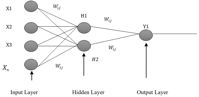
Figure 1: Structure of a Multilayer Feed-Forward Neural Network.
Y1 X1
X2
X3
H1
Where;
= Output variable
= Input variable
= Weights between layers
= Hidden layer containing activation/ Transfer function
Mathematically,
F(x) = = )
The neural network can be used for linear programming optimization problems by using the
structure above to relate with the LP equation; A back propagation algorithm will be used to
teach the neural network on solving the optimization problems.
3.3 Training of Artificial Neural Network
In setting up the neural network for training, the data had to be arranged in the form of input
variables and output variables. For this case of linear programming as seen in figure 3.1,
eleven (11) input variables and three (3) output variables were used to train the network. The
number of neurons used for the training of the network was set at 50 neurons, this enables the
weight (W) and bias (b) of each neuron to be adjusted to suit the size of the network.
Figure 2: Structure of the Network with the Input and Target Variables (MATLAB).
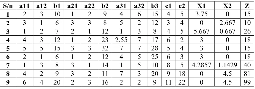
Table 1: Training, Testing and Validation Data Set (sample).
S/n a11 a12 b1 a21 a22 b2 a31 a32 b3 c1 c2 X1 X2 Z
1 2 3 10 1 2 9 4 6 15 4 5 3.75 0 15
2 3 1 6 3 3 8 5 2 12 3 4 0 2.667 10
3 1 2 7 2 1 12 1 3 8 4 5 5.667 0.667 26
4 4 3 12 1 2 23 2.55 7 17 6 2 3 0 18
5 5 5 15 3 3 32 7 7 28 5 4 3 0 15
6 2 1 6 1 2 12 4 5 25 6 3 3 0 18
7 1 3 8 3 1 14 1 5 10 8 5 4.2857 1.1429 40
8 4 2 9 3 2 11 7 3 20 9 18 0 4.5 81
A data set of about 140 linear programming problems were used in training the neural
network to be able to adjust and predict solutions in the format of a linear programming
problem with two (2) variables and three (3) constraints equations. In table 1, the sample of
training, testing and validation data can be seen. Also appendix G contains complete training,
testing and validation data set.
3.4 Data Collection Source
The data for this project work was collected from Patrich Global Enterprise. Patrich Global
Enterprise (PGE) is a soap manufacturing Company located in Rivers State, Nigeria. The
Company specializes in the production of cosmetics and different kinds of soap. For the
purpose of this project, the soap production will be the area of concentration.
The data collected are based the following categories of raw materials required for the
production of soap which are:
i. Oils (kernel oil, palm oil),
ii. Sodium compounds (Sodium Hydroxide, Sodium Carbonate & Sodium Sulphate) and
iii. Additives (fragrance, menthol and color).
These materials are passed through the following processes; Chemical Preparation, Drying
and Packaging. The production data for January 2018 to June 2018 As seen below.
For the input data
Let the number of laundry soap to be produced each month = and bathing soap to be
produced each month = ,
Max Z = (3.10)
Subject to;
<= (3.11)
<= (3.12)
After substituting the various values into the equations above, we get the following for the
month of January
Optimize (Max) Z = 65 + 75 (3.14)
Subject to:
10 + 8 <= 7500 (3.15)
17 + 12 <= 12000 (3.16)
0.5 +0.7 <= 400 (3.17)
For the Month of February
Optimize (Max) Z = 70 + 80 (3.18)
Subject to:
15 + 12 <= 10000 (3.19)
20 + 15 <= 15000 (3.20)
0.9 + <= 500 (3.21)
For the Month of March
Optimize (Max) Z = 75 + 95 (3.22)
Subject to:
30 + 14 <= 15000 (3.23)
15 + 10 <= 11000 (3.24)
0.45 + 0.85 <= 450 (3.25)
For the Month of April
Optimize (Max) Z = 75 + 95 (3.26)
Subject to:
22 + 15 <= 12000 (3.27)
27 + 18 <= 25000 (3.28)
0.57 + 0.92 <= 359 (3.29)
For the Month of May
Subject to:
20 + 18 <= 12400 (3.31)
16 + 20 <= 18000 (3.32)
0.5 +0.6 <= 435 (3.33)
For the Month of June
Optimize (Max) Z = 85 + 110 (3.34)
Subject to:
19 + 14 <= 10000 (3.35)
25 + 25 <= 20000 (3.36)
0.7 + 1.2 <= 500 (3.37)
The above equations are converted into linear programming model as shown in a table format
on Table 8. This enables the Artificial Neural Network to understand the various inputs in a
tabular form in the same manner of the training data sample.
Table 8: Data for Soap Production for the Months of January to June in Linear Programming Form.
S/n
1 10 8 7500 17 12 12000 0.5 0.7 400 65 75 2 15 12 10000 20 15 15000 0.9 1 500 70 80 3 30 14 15000 15 10 11000 0.45 0.85 450 75 95 4 22 15 12000 27 18 25000 0.57 0.92 359 75 95 5 20 18 12400 16 20 18000 0.5 0.6 435 80 100 6 19 14 10000 25 25 20000 0.7 1.2 500 85 110
IV. RESULTS AND DISCUSSION
4.1. Neural Network Optimization Results for Maximum Profit
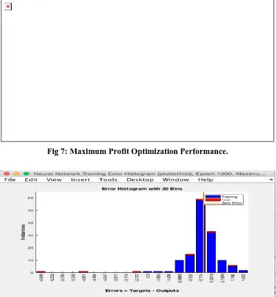
During the Maximum Profit Optimization, the convergence point started at around 300th
epoch and best performance occurred around the 656th epoch (as seen on Figure 7) with the
performance value at 0.92233. This was the convergence point where the best results for the
optimization was gotten for the Bathing Soap production.
The errors from the Maximum Profit Optimization (as seen on figure 8) can be also had 20
bars (bins) of errors. It also was observed that the errors were high during the training process
Fig 7: Maximum Profit Optimization Performance.
Fig 8: Maximum Profit Optimization Errors.
4.4. Comparing Results of Artificial Neural Network Solution with Simplex Method The neural Network was able to optimize soap production and the maximum profit for each
month can be seen on table 7. From the optimized results gotten, the corresponding values
were compared with by solving the same problems using the simplex method.
The simplex method was also used to optimize the system. The Company’s production data
Table 7: Company Profit, Results from Simplex Method and Optimization Results from Artificial Neural Network for the Months of January to June 2018.
Month Company Profit(₦) Maximum Profit (₦) (Simplex Method)
Maximum Profit (₦) (Neural Network Method)
January 30,000 49800 49830.9972
February 28700 40000 39998.0210
March 30625 58500 58544.0084
April 47000 56800 56832.0183
May 46800 68888.89 68888.9075
June 47200 53846.15 53840.1682
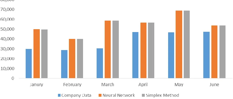
Figure 9: Comparison of Results from Company Data, Neural Network and Simplex Method for Maximum Profit from Production of Both Laundry and Bathing Soap.
For each month during optimization, it was observed that the maximum profit was more than
the Company’s recorded profit. This shows that the profit being generated from the Company
for these months was not the maximum attainable profit from production as seen on Figure 9.
It was observed that maximum profit prior to this optimization process was at ₦47,200 at the
same cost per unit of each soap. After optimization was done, the maximum projected profit
was approximately ₦69,000 which is about a 47% increase in maximum profit from current
production data.
V. CONCLUSION
From this project, Artificial Neural Network was modelled and used to optimize soap
achieve up to 1000 iterations where the error values between the targets and output became
lowest.
After Optimization with the Artificial Neural Network, solutions from simplex method of
solving linear programming problems was used to compare with the results from the
Artificial Neural Network to confirm and ascertain the optimized results. After the
comparison of results, it was observed that the both (Neural Network and Simplex) results
were over 98% percent in similarities.
The maximum projected profit was also effected with a 47% increase in profit from ₦47,200 to ₦69,000 in a month. However, production of bathing soaps will be more profitable in
production than laundry soaps. More resources should be put into the production of bathing
soaps for higher profit margins.
VI. REFERENCES
1. Abdulkareem, K., F., H., & Fath, A., F., K., Artificial Neural Network Implementation
for Solving Linear Programming Models. Journal of Kufa for Mathematics and
Computer, 2014; 2(1): 113-121.
2. Fogel, D., Liu, D. & M., Keller., Introduction and Single‐Layer Neural Networks, 2016; 5-34.
3. Kourosh, R., Farhang, K., N., Reza, H., Hamid, R., S. & Ebrahim, A., Solving Linear
programming problems. Singaporean Journal of Business Economics, and Management
Studies, 2013; 1(10).
4. Lilly, M. T., Ogaji, S. & Probert, S., D., Manufacturing: Engineering, Management and
Marketing. (Eds.), Partridge. China, 2015; 1st edition: 100-125.
5. Mirza, C., Neural Networks and Back Propagation Algorithm, Institute of Technology
Blanchardstown, Blanchardstown Road North Dublin 15 Ireland. Unpublished, 2010.
6. Raul, R., Neural Networks: A Systematic Introduction, 2005; Retrieved March 30, 2018,
from http://www.statsoft.com/textbook/neuralnetworks/apps, 2018.
7. Sharma, J., K., Operations Research Theory and Applications. (Eds.), Macmillan, India,