Review Of Self-Tuning Controller And Its Application In Electrical Power System

137 _______________________

 Rudy Gianto is currently with Department of Electrical Engineering, Tanjungpura University, Indonesia, Phone: +62 (561) 740186. E-mail: [email protected]

Review Of Self-Tuning Controller And Its

Application In Electrical Power System

Rudy Gianto

Abstract: Self-tuning controller (STC) is one of the techniques of adaptive control. The controller is called self-tuning, since it has the ability to adjust its own parameters according to the system conditions to obtain satisfactory control performance. This adaptive controller is developed to overcome the shortcomings of the non-adaptive controllers. This control technique is very popular, and has been implemented in many important engineering applications. One important application of STC is in the field of electrical power engineering, where the STC concept has been employed to design the self-tuning stabilizer for damping of power oscillation. This paper provides an overview on the self-tuning controller and its application in improving dynamic performance of an electrical power system.

Index Terms: Adaptive cotroller, Self-tuning controller, dynamic performance, power system, Kalman filtering.

————————————————————

1 I

SELF-TUNING controller was originally proposed by Kalman in 1958. However, because of the unavailability of high-speed computers and inadequately developed theory, this technique was not taken up seriously at that time. The breakthrough came with the work reported by Astrom and Wittenmark in 1973. Since then this technique has become popular, especially due to the advent of microprocessors, which make it feasible to implement the STC algorithms [1]. Self-tuning controller (STC) is one of the techniques of adaptive control. This adaptive controller is developed to overcome the shortcomings of the adaptive controllers. The non-adaptive (fixed-parameter) controller is, in general, based on one particular system operating condition. The key disadvantage of this controller is that the possibility of the controller performance deterioration under other operating conditions. Furthermore, it is not possible to achieve maximum performance for each and every operating condition when the controller parameters are fixed. Recently, adaptive control techniques have been proposed to overcome the disadvantage of fixed-parameter controllers design. In this adaptive controller design, the controller parameters are determined online and adaptive to the changing in system operating conditions. This paper provides an overview on the self-tuning controller [2-9]. Previous works published in the area of adaptive damping controller designs using self-tuning controller concept are also presented in this paper [10-19].

2 SELF-TUNING CONTROLLER

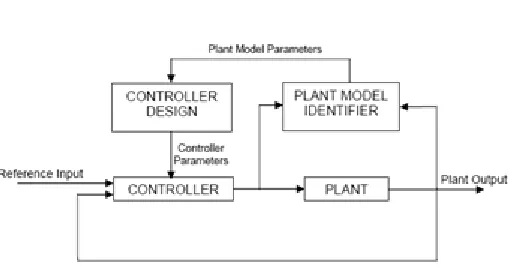
STC can be thought of as having two loops (see Fig. 1): an inner loop consisting of a conventional controller (but with varying parameters), and an outer loop consisting of a plant model parameters identifier and a controller design with the function of adjusting the controller parameters. The controller design block diagram in Fig. 1 represents an online solution to a design problem for a system with known parameters [1-3].

Fig. 1 Self-tuning controller

In the context of control theory applied in general to self-tuning controller, the methodologies which can be used for controller design include: linear quadratic, minimum variance, gain-phase margin design, pole assignment (pole placement) and pole shifting. Whereas, those for plant model parameters identification schemes include: squares, recursive least-squares and Kalman filtering [1-3]. In [10-19], the STC has been applied to design the power system oscillation damping controller. In [10-17], the recursive least square (RLS) method has been used to identify the system parameters online. Whereas, in [18, 19], the Kalman Filter (KF) was used for the plant identification. Furthermore, the pole shifting algorithm has been employed in [10-19] for controller design to determine the controller parameters. The overview on RLS method, Kalman filter and pole shifting algorithm which have been proposed for power systems applications are given in the following.

2.1 RLS Parameters Identification Method

In STC, the model of the system to be controlled is usually described by a linear difference equation, and the model parameters are identified every sampling interval. The system model in the discrete-time domain is assumed to be of the form [1, 3-4]:

) ( )

( ) ( ) (

) ( )

( ) ( ) (

) ( )

( ) ( ) (

g n

2 1

b n

2 1

0

h n

2 1

n n g 2 n g 1 n g n

n n u b 2 n u b 1 n u b n u b

n n y h 2 n y h 1 n y h n y

g b h

           

 

     

 

    

  

(1)

138 model parameters to be identified;  is a sequence of

independent and equally distributed random noise, and n is the sampling instant. The operator notation will be used here

for conveniently writing the difference equation (1). Let qk be the backward shift (or delay) operator which is used to relate [1]:

qky(n)y(nk) (2)

On using (2), (1) can be rewritten as:

H(q1)y(n)B(q1)u(n)G(q1)(n) (3)

where:

g g

b b

h h

n n 2

2 1 1 1

n n 2 2 1 1 0 1

n n 2 2 1 1 1

q g q

g q g 1 q G

q b q

b q b b q B

q h q

h q h 1 q H

 

 

 

 

 

 

  

 

    

    

  

) (

) (

) (

(4)

The estimation of the model parameters can be simplified by assuming G(q1)1 which modify (3) to become [1]:

H(q1)y(n)B(q1)u(n)(n) (5)

Equation (5) can be expressed in terms of the various model parameters as the following:

) ( ) ( )

( ) ( ) (

) ( )

( ) ( ) (

n n n u b 2 n u b 1 n u b n u b

n n y h 2 n y h 1 n y h n y

b n

2 1

0

h n

2 1

b h

   

     

 

    

 

(6)

By introducing the parameter and regression vectors:









T n 1 0 n 2

1

b n n u 1 n u n u h n n y 2 n y 1 n y

b h

n

b b b h h

h n

) ( ) ( ) ( ) ( ) ( ) ( ) (

) (

 

     

 

 

 

Φ Θ

(7)

Equation (6) can be rewritten in a compact form, using definitions in (7):

y(n)Φ(n)TΘ(n)(n) (8)

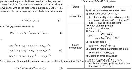
The parameter vector Θ is to be estimated from the observations of system inputs and outputs. In adaptive controllers, the observations are obtained sequentially in real time. It is then desirable to make the computations recursively to reduce computing time. Computation of the least-squares estimate is arranged in such a way that the results obtained at time n-1 can be used to get the estimates at time n. In recursive implementations of the least-squares method, the computation is started with known initial conditions and uses the information contained in the new data samples (from the measurements) to update the old estimates. The RLS algorithm for estimating model parameters hi and bi is summarized in the following (see Table 1).

Table 1

Summary of the RLS algorithm

Stage Description

Initialisation

1) Model parameters estimates: Θˆ(0)

2) Error covariance: P(0)_cI

(I is the identity matrix which has the dimension of (nh+nb+1) (nh+nb+1),

and c is a specified constant)

Online computation

For each sampling instant: n = 1, 2,…., calculate: 1) Gain vector:

) ( ) ( ) (

) ( ) ( )

(

n 1 n n

n 1 n n

T

f Φ P Φ

Φ P K

 



 

2) Prediction error:

(n)y(n)Φ(n)TΘˆ(n1)

3) Update of model parameter estimate: Θˆ(n)Θˆ(n1)Κ(n)(n)

4) Update of error covariance:

P(n)





f is the forgetting factor which has

the value of 0_f 1)

2.2 Kalman Filter (KF) State Estimation

KF is essentially a set of mathematical equations that provides an efficient computational (recursive) means to estimate the state of a process [6]. KF uses a recursive algorithm whereby the updated estimate of the state at each time step is computed from the previous estimate and the new input data, so only the previous estimate requires storage [5-9]. KF provides a unifying framework for the derivation of an important family of adaptive filters known as recursive least-squares filters [6]. KF addresses the problem of estimating the state of a linear discrete-time dynamical system governed by the following equation [5-9]:

x(n1)Ax(n)w_x(n) (9)

y(n)Cx(n)w_y(n) (10)

where: x is the state vector to be estimated; y is the observation vector which contain a set of observed (measured) data; wx and wy are the process and

measurement noise respectively; A is the state transition matrix, and C is the measurement matrix. The noise vector sequences wx(n) and wy(n) in (9) and (10) are assumed to be

known and independent (of each other). It is also assumed that they are white (uncorrelated) noise, with zero mean and covariance matrix defined by:

E[w_x(n)w_x(n)T]Q(n) (11)

E[w_y(n)w_y(n)T]R(n) (12)

139 noise covariance matrix Q and measurement noise covariance

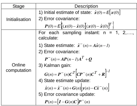
matrix R might change with each time step, however, it will be assumed here that they are pre-specified constants [6]. The state matrix A in (9) relates the state of the system at time n+1 and n, whereas, the measurement matrix C in (10) relates the state to the measurement y. For a time-varying system, matrices A and C change with each time step. Suppose that a measurement on a linear discrete-time dynamical system described by (9) and (10) has been made at sampling instant n. The requirement is to use the information contained in the new measurement y(n) to update the estimate of the unknown state x(n). The KF recursive algorithm for state estimation is summarised in Table 2.

Table 2

Summary of the KF algorithm

Stage Description

Initialisation

1) Initial estimate of state: xˆ(0)E





2) Error covariance:

P(0)E











Online computation

For each sampling instant: n = 1, 2,…., calculate:

1) State estimate: xˆ(n)Axˆ(n1)

2) Error covariance:

P(n)AP(n1)ATQ

3) Kalman gain:

G(n)P(n)CT





4) State estimate update:

xˆ(n)xˆ(n)G(n)





5) Error covariance update:

P(n)





It is interesting to note that, when model parameters are time-varying, the model described by (8) can be interpreted as a linear state-space model of the form [1, 2, 4]:

) ( ) ( ) ( ) (

) ( ) ( ) (

n n n n y

n n 1 n

T _



   

Θ Φ

Θ Θ

(13) The above observation shows that the least-squares estimate can be interpreted as a KF for the process described by (13). It is possible to express (13) in the form in (9) and (10), when

T

,C Φ I

A  and x is the plant model parameters vector, to obtain [1, 2, 4]:

) ( ) ( ) ( ) (

) ( ) ( ) (

n n n n y

n n 1 n

T _



   

x Φ

x x

(14)

With the plant model in (14), the KF algorithm in Table 2 can be for model parameters determination.

2.3 Pole-Shifting Controller Design

In the pole-shifting controller design, it is assumed that the pole characteristic polynomial of the closed-loop system has the same form (i.e. the same order) as the pole characteristic polynomial of the open-loop system, but the pole locations determined by the roots of the characteristic polynomial are shifted by a factor s [10-19]. Fig. 2 shows the control system

block diagram for illustrating the pole-shifting controller design procedure. The system to be controlled in Fig. 2 has the transfer function of the form:

) (

) ( ) (

1 1 1

z

q H

q B q

G _



 _{ (15)}

where H(q-1) and B(q-1) are polynomials defined by (4). The transfer function of the controller is assumed to be of the form:

) (

) ( ) (

1 1 1

z

q D

q C q

K _



 _{ (16)}

where C(q-1) and D(q-1) are polynomials given by:

d d

c c

n n 2

2 1 1 1

n n 2 2 1 1 0 1

q d q

d q d 1 q D

q c q

c q c c q C

 

 

 

 

    

    

 

) (

) (

(17)

With the plant output y in Fig. 2 representing the deviation from a given operating point, the reference r input to the closed-loop system takes the value of zero as shown.

It can be shown that the pole characteristic polynomial of the closed-loop system in Fig. 2 is:

P(q1)H(q1)D(q1)B(q1)C(q1) (18)

In the pole-shifting method, the pole characteristic polynomial of the closed-loop system P(q-1) has the same form as the pole characteristic polynomial of the open-loop system H(q-1) but the pole locations are shifted radially towards the origin of unit circle in the z-plane by a factor s 0s1 [4,15,18]. Thus the following equation holds:

H(q1)D(q1)B(q1)C(q1)H(_sq1) (19)

where:

h

h

h n

n n s 2

2 2 s 1 1 s 1

sq 1 hq h q h q

H(  )       (20)

Fig. 2 Closed-loop control system

Expanding both sides of (19) and comparing the coefficients with the same power of q-i will result in the linear equation system which must be solved to obtain the controller parameters ci and di. In order to guarantee that the solution of

the linear equation system is unique, it has been suggested in [48] that the number of the parameters nc and nd should be

1

n_h and n_b1 respectively. In partitioned vector/matrix forms, the formulation of the linear equation system for

) n

(and

_c n n n 1

n n

140                                2 Z 1 Z 2 Z 1 Z 4 Z 3 Z 2 Z 1 Z L L R R M M M M        (21)

where matrices K K K G nG nK

3 Z n n 2 Z n n 1

Z   M   M  

M , ,

K G G K G G n 2 Z n 1 Z n 2 Z n 1 Z n n 4

Z   R  R  L  L 

M , , , and

are given by:

                                      0 3 n 2 n 1 n 0 1 2 0 1 2 Z 4 n 3 n 2 n 1 2 1 1 Z b b b b 0 b b b 0 0 b b 1 h h h 0 1 h h 0 0 1 h 0 0 0 1 G G G G G G                  M M                                         G G G G G G G G G G G G G n 3 n 2 2 n n 1 2 n 1 n n 4 Z n 3 n 2 1 n n 1 2 n 1 n 3 Z b 0 0 0 b b 0 0 b b b 0 b b b b h 0 0 h h 0 h h h h h h                  M M                                                                   0 0 0 1 h 1 h 1 h c c c d d d 2 Z n s n 2 s 2 s 1 1 Z n 1 0 2 Z n 2 1 1 Z G G K K     L L R R ; ) ( ) ( ) ( ;

It is to be noted that in (21), the model parameters hi and bi are

identified every sampling instant by using one of the system identification methods described in Sections 2.1 and 2.2.

3 A

STC

P

S

In [10-17], the STC concept has been employed to design the self-tuning PSS for damping of power oscillation. In the design, the recursive least square method was used to estimate the system parameters online. Based on the

identified system parameters, the pole-shifting algorithm has been incorporated in the controller design to determine the controller parameters. A similar approach has been applied to a TCSC damping controller in [18, 19]. In [18, 19], Kalman Filter (KF) has been used for parameters identification method, and pole shifting algorithm was employed in the controller design. Furthermore, the self-searching and self-optimising pole shifting techniques have been incorporated in the controller design in [10-19]. The techniques have been used in the design with the objective to enable the modification of the pole shifting factor with respect to control signal to avoid unsatisfactory control performances. With these techniques, excessive pole shifting is no longer a problem. Thus, the control constraints violation and control signal saturation which might affect the control performances can be avoided and the control signals are kept within their limits. Results presented in [10-19] indicate that the proposed self-tuning damping controller can provide good damping under varying operating conditions and different disturbances. Although the results presented in [10-19] indicate that the proposed self-tuning damping controller can provide good damping under varying operating conditions and different disturbances, some issues have been identified in the application as the following:

- Low-order system model has to be used in the application of the method due to computation time requirement (higher order model requires longer computation time which is not suitable for online implementation). Also, it appears that there is no systematic technique for determining the order of the system model (i.e. na and nb). In [10-17], the third order

system model has been selected to approximate the higher order power system. This approximation might lead to some errors and affect the system identification and controller design. Furthermore, there is no guarantee that the low-order model will be sufficient to track the important system dynamics and modes of interest.

- It is difficult to implement the method in [10-19] for system having multiple modes of oscillations, and it will be more difficult if the modes of interest have to be simultaneously considered in the application of the method.

- Coordination amongst multiple damping controllers is very important for achieving optimal oscillation dampings in multi-machine power system. It is not clear how the controllers coordination can be implemented in the approach proposed in [10-19]

4 C

This paper has presented and discussed the popular adaptive control technique namely self-tuning controller. This adaptive controller is developed to overcome the shortcomings of the non-adaptive controllers. The application of the adaptive controller in enhancing power system dynamic performance has also been presented in the paper.

APPENDIX

A.1 Expectation

If X is a discrete random variable with the possible values n

2

1 x x

141 







n

1

i i i

x X P x X] [

E (A.1)

In words, the expected value of X is a weighted average of the possible values of X, each value is weighted by its probability (P).

A.2 Variance

If X is a random variable with mean  then the variance of X, denoted by Var(X), is defined by [20-21]:

Var(X)E[(X)2] (A.2)

An alternative formula for Var(X) can be expressed as follows [20]:

Var(X)E[X2](E[X])2 (A.3)

or, in words, the variance of X is equal to the expected value of the square of X minus the square of the expected value of X.

A.3 Covariance

The covariance of two random variables X and Y, denoted by Cov(X,Y), is defined by [20-22]:

Cov (X,Y)E[(X_x)(Y_y)] (A.4)

where _xE[X] and _yE[Y] are the mean values of X and Y respectively. A useful expression for Cov(X,Y) can be obtained by expanding the right side of (A.4) which yields:

Cov (X,Y)E[XY]E[X]E[Y] (A.5)

From the definition of covariance, it can be seen that covariance satisfies the following property [20]:

Cov (X,Y)Cov (Y,X) (A.6)

Another important property of covariance is that, if X and Y are independent [22]:

E[XY]E[X]E[Y] (A.7)

From (A.5) and (A.7) it can be concluded that, if X and Y are independent, the covariance of the two random variables is given by:

Cov (X,Y)0 (A.8)

A.4 Covariance Matrix

Covariance matrix is a matrix of covariances between elements of a vector. Consider a random vector X (where each component of the vector Xi is a random variable):

X





Then, the covariance matrix S is the matrix where its component is given by [22]:

S_ijCov (X_i,X_j)E[(X_i_i)(X_j_j)] (A.10)

Due to symmetry property of covariance (see (A.6)), the covariance matrix is always a symmetric matrix (i.e. S_ij S_ji). Also, based on (A.2) and (A.4), the covariance of any component Xi with itself is the variance of the component:

Cov (Xi,X_i)E[(X_i_i)2]Var(X_i) (A.11)

R

[1] Chalam, V.V.: Adaptive Control Systems: Techniques and Applications, Marcel Dekker, New York, 1987.

[2] Astrom, K.J., and Wittenmark, B.: Adaptive Control, Addison-Wesley Publishing Company, 1995.

[3] Sastry, S., and Bodson, M.: Adaptive Control: Stability, Convergence, and Robustness, Prentice-Hall, New Jersey, 1989.

[4] Ljung, L., and Soderstrom, T.: Theory and Practice of Recursive Identification, MIT Press, Cambridge-London, 1987.

[5] Haykin, S.: Adaptive Filter Theory, Prentice-Hall, New-Jersey, 1996.

[6] Welch, G., and Bishop, G.: An Introduction to the Kalman

Filter, available online at

http://www.cs.unc.edu/~welch/kalman.

[7] Zaknich, A.: Principles of Adaptive Filters and Self-Learning System, Springer-Verlag, London, 2005.

[8] Haykin, S.: Kalman Filtering and Neural Network, John Wiley & Sons, 2001.

[9] Brown, R.G.: Introduction to Random Signal Analysis and Kalman Filtering, John Wiley & Sons, 1983.

[10]Ghosh, A., Ledwich, G., Malik, O.P., and Hope, G.S.: ‘Power system stabilizer based on adaptive control techniques’, IEEE Trans. Power Apparatus and Systems, 1984, 103, (8), pp. 1983-1989.

[11]Cheng, S., Malik, O.P., and Hope, G.S.: ‘Self-tuning stabiliser for a multimachine power system’, IEE Proceedings-C, 1986, 133, (4), pp. 176-185.

[12]Cheng, S., Chow, Y.S., Malik, O.P., and Hope, G.S.: ‘An adaptive synchronous machine stabilizer’, IEEE Trans. Power Systems, 1986, 1, (3), pp. 101-109.

[13]Pahalawatha, N.C., Hope, G.S., Malik, O.P., and Wong, K.: ‘Real time implementation of a MIMO adaptive power system stabiliser’, IEE Proceedings-C, 1990, 137, (3), pp. 186-194.

142 simulation and implementation studies’, IEEE Trans.

Energy Conversion, 1991, 6, (2), pp. 310-319.

[15]Malik, O.P., Chen, G.P., Hope, G.S., Qin, Y.H., and Xu, G.Y.: ‘Adaptive self-optimising pole shifting control algorithm’, IEE Proceedings-D, 1992, 139, (5), pp. 429-438.

[16]Chen, G.P., Malik, O.P., Hope, G.S., Qin, Y.H., and Xu, G.Y.: ‘An adaptive power system stabilizer based on the self-optimizing pole shifting control strategy’, IEEE Trans. Energy Conversion, 1993, 8, (4), pp. 639-645.

[17]Kothari, M.L., Bhattacharya, K., and Nanda, J.: ‘Adaptive power system stabiliser based on pole-shifting technique’, IEE Proc.-Gener. Transm. Distrib., 1996, 143, (1), pp. 96-98.

[18]Sadikovic, R., Korba, P., Andersson, G.: ‘Self-tuning controller for damping of power system oscillations with FACTS devices’, IEEE PES General Meeting, June 2006.

[19]Korba, P., Larsson, M., Chaudhuri, B., Pal, B., Majumder, R., Sadikovic, R., and Andersson, G.: ‘Towards real-time implementation of adaptive damping controllers for FACTS devices’, IEEE PES General Meeting, June 2007, pp.1-6.

[20]Ross, S.M.: Introduction to Probability and Statistics for Engineers and Scientists, Elsevier Academic Press, 2004.

[21]Gordon, H.: Discrete Probability, Springer-Verlag, New York, 1997.