Article
Modeling and Analyzing Multi-tier Millimeter/Micro
Wave Hybrid Caching Networks
Jihong Zhao 1,2, Shuyuan Zhao 1,*, Hua Qu 1, and Gongye Ren 1
1 School of Electronic and Information Engineering, Xi’an Jiaotong University, Xi’an, 710049, China 2 School of Telecommunication and Information Engineering, Xi’an University of Posts And
Telecommunications, Xi’an 710061, China
* Correspondence: [email protected]; Tel.: + 86-15829397833
Abstract: In the fifth generation communication system, millimeter wave (mmWave) networks will coexist with traditional micro wave (μWave) networks, which allows for higher data transmission rate and better user experience. In this paper, we give a comprehensive framework of mathematical models and analytical methods for multi-tier mmWave and μWave hybrid caching networks based on stochastic geometry. We propose an association strategy by assuming average biased-received power association and Rayleigh fading. Accordingly, by using a D-ball approximating blockage model of mmWave networks, expressions of the cell association probability and the coverage probability of the hybrid networks are derived. Also, we use the average successful delivery probability as the performance metric to analyze the existing caching placement strategies. Simulation results validate the accuracy of our analytical conclusions.
Keywords: Multi-tier hybrid caching networks; stochastic geometry; millimeter wave; average successful delivery probability; performance analysis
1. Introduction
Over the past several years, the global mobile data traffic grows rapidly with the proliferation of smart phones, portable devices, etc., and is expected to increase to 30.6 exabytes per month by 2020 [1]. With the increasing demand for higher capacity and lower latency in wireless networks, the fifth generation (5G) communication system has been proposed to improve the capacity of current networks by a factor of 1000 [2]. However, limited micro wave (μWave) spectrum does not seem to be able to meet this increasing demand in the near future. Therefore, the large available millimeter wave (mmWave) spectrum, ranging from 30GHz to 300GHz, is becoming attractive for 5G cellular networks, and has been considered to be the key to an order of magnitude increase in the capacity of current cellular networks [3–6].
There are several distinctive features of mmWave cellular networks different from μWave cellular networks due to the particular channel characteristics and hardware constraints [7] at mmWave frequencies: (1)large number of antennas. Since the antenna sizes decrease as the wavelength decreases, mmWave signals enable very high dimensional antenna arrays for further gains via beamforming and spatial multiplexing [8]. Therefore, mmWave cellular networks can be considered as noise-limited rather than interference-limited [9–11]. (2)complex propagation environment. MmWave signals are more sensitive to blockage effects than microwave, as certain materials like outer birck walls found on building exteriors cause severe penetration loss [12]. The isolation effects of walls indicate that indoor users are unlikely to be covered by outdoor mmWave base stations (BSs). Three different states of the mmWave path loss and blockage models, namely line-of-sight (LOS), non-line-of sight (NLOS) and outage states, have been studied in recent literatures [10,11]. For analytical tractability, literature [13] proposed equivalent LOS ball model. In [8], a probabilistic LOS ball model was considered and it is generalized to a two-ball model based on the path loss intensity matching algorithm in [11]. Recently, a more general D-ball
approximation model was used to analyze SINR coverage probability for K -tier heterogeneous mmWave cellular networks in [14].
Hence, to alleviate the spectrum crunch and meet the increasing data rate demands, mmWave networks will coexist with traditional μWave networks in future 5G networks. In several recent studies such as [8], [14] and [15], hybrid network scenarios have been considered, and mmWave small cells are opportunistically used, which means that the user equipments (UEs) are offloaded to the μWave networks when it is not possible to establish a mmWave connection. In [16], the authors considered an mmWave network overlaid μWave network, and the work in [15] provided uplink and downlink coverage analysis of hybrid networks.
On the other hand, studies in recent years show that a large portion of mobile data traffic is generated by repeated request of numerous popular contents [17] and the storage capacity of memory devices grows rapidly at a relatively low cost. So content caching has attracted much attention as a method of offloading mobile data traffic, improving the throughput and reducing the latency in cellular networks, without requiring additional bandwidth [18,19].The role of caching technology in 5G wireless network is demonstrated in [20,21], and key notions, challenges, and research topics of wireless caching were provided in [22]. Performance analysis of wireless caching networks was investigated in [23–26]. The work in [23,24] analyzed the outage probability of cache-enabled networks with/without underlying macro cellular network respectively, in which the BS locations are assumed to be distributed as homogeneous Poisson point processes (PPPs). The performance of wireless caching helper networks consisting of caching helpers whose locations are modeled as PPPs was analyzed in [25,26]. Yang et al. [27] derived the average ergodic rate and outage probability for a reference user in cache-enabled heterogeneous networks with push-based content access protocol. However, most of the previous works only considered caching scenario in the μWave heterogeneous networks.
In this paper, we propose an analytical framework based on stochastic geometry for modeling and analyzing the multi-tier mmWave/μWave hybrid caching networks, with two pre-fetching strategies called random caching strategy (RCS) and popularity-base caching strategy (PCS). Our main contributions can be summarized as follows:
A general system model of the multi-tier mmWave/μWave hybrid caching networks is established, where BSs in each tier are randomly located and have a particular carrier frequency, transmit power, path loss exponent, spatial density, and bias towards admitting UEs. Also, we propose the mmWave/μWave association rule and the caching strategies.
Considering the D-ball blockage model of the mmWave networks, which is similar to the piece-wise LOS probability function approach proposed in [28], we derive the cell association probability of the multi-tier hybrid networks by assuming average biased-received power association. Moreover, for simplicity and tractability, we consider the noise-limited scenarios for the mmWave networks and the interference-limited scenarios for the μWave networks with Rayleigh fading, and give the general analytical expressions.
We use the average successful delivery probability (ASDP) as the performance metric for the hybrid caching networks, and evaluate the performance of two aforementioned pre-fetching strategies. Simulation results demonstrate the accuracy of our analysis.
This paper is organized as follows: In Section 2, we describe the system model of the multi-tier mmWave/μWave hybrid caching networks, including mmWave network model, μWave network model, association strategy and caching model. Also we derive the general expressions of tier association probability of the multi-tier hybrid networks. In Section 3, we consider the ASDP as the performance metric to analyze the different caching strategies and provide the final results. In Section 4, we compare analytical results with the Monte Carlo simulation results. Finally, Section 5 provides our conclusions. Several proofs are relegated to the Appendix.
In this section, we consider a multi-tier heterogeneous downlink mmWave/μWave hybrid caching network comprised of a Km-tier mmWave network and a K-tier μWave network. The
th
k tier mmWave network is distributed as a homogeneous PPP m k
of density m k
(k1, 2,...,Km), and the th
k tier μWave network is distributed as a homogeneous PPP k
of density k
(k1, 2,...,K ). Also, the UEs in the network are spatially distributed as an
independent homogeneous PPP u of density u, and are assumed to be equipped with two sets
of antennas to receive mmWave and μWave signals respectively. A typical UE is assumed to be located at the origin according to Slivnyak’s theorem [29] without loss of generality. In a cache-enabled hybrid network, the performance of caching depends on the density of BSs, cache size, content request probability, caching strategy, propagation environment, etc.
2.1. MmWave Network Model 2.1.1. Beamforming Model
The antenna gains of mmWave BSs and UEs are modeled according to the sectorized antenna model [30], given by
0 0
| | ( )
| |>
M
m
G if
G
G if
, (1)
where 0 denotes the beam-width or main lobe width, GM and Gm are the array gains of main
and side lobes, respectively. Therefore, the effective antenna gain between the typical user and mmWave BSs can be described by
2 0
0 0 2 0
2 2 2
2 2 2
2
M M MM
M m Mm
m m mm
G G p
G G G p
G G p
, (2)
where pij with i j,
M m,
is the probability of the antenna gain G Gi j seen by the typical UE.In this paper, for simplicity and tractability of analysis, we assume that the BS and UE antennas are perfectly aligned and the beamforming gain is always G G G M M.
2.1.2. Blockage Model
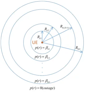
MmWave signals are more sensitive to blockages, and the link between a typical UE and its associated mmWave BS can be in LOS, NLOS or outage state [10]. Define p r( ) as the probability that the arbitrary link of length r is in LOS state, and it can be approximated by step functions, which provide tractable and accurate results according to [28,31]. In this paper, we adopt the D-ball approximation model proposed in [14]. As shown in Figure 1, in a Km-tier mmWave network, for
the kth tier ( 0,1,..., m
k K ), a link is in LOS state with probability p r( )k1 inside the first ball
with radius Rk1, while NLOS state occurs with probability 1k1. Similarly, the LOS probability is
( ) kd
p r when the link length r is between Rk d( 1) and Rkd for d2,...,D, and when rRkD,
Figure 1. The D-ball model for the mmWave network. So, the path loss function of the kth tier can be expressed as follows:
1 1
2 2
1 0 1 0 1
2 0 2 0 1 2
0 0 ( 1)
(1 ) if 0, (1 ) if , ( ) ...
(1 ) if , outage if
L N
k k
L N
k k
L N
kD kD
L N
k k k
L N
k k k k
k
L N
kD kD k D kD
kD
L r L r r R
L r L r r R R
L r
L r L r r R R
r R
, (3)
where L kd
and N kd
denote the LOS and NLOS path loss exponents for the dth ball in the kth
tier, respectively, 0
L
L and 0
N
L are the path loss of LOS and NLOS links at a unit distance (typically about
24 / m , where m denotes the mmWave wavelength), and Rkd is the radius of the th
d ball of the kth tier.
For characterizing the downlink signal-to-interference-plus-noise ratio (SINR) distribution, the point process formed by the path loss between the typical UE at origin and BSs in the kth tier is
defined as: k
L r rk( ) | k
[8]. By using the void probability theorem of PPPs [32], thecomplementary cumulative distribution function (CCDF) of L rk( ) is given in [14]:
L rk( )x
exp
k
0,x
, (4)
and
2 2
0 1
1
2/ 2
0 1 0 1 0
2 2
0 1
2/ 2
0 1 0 1 0
0,
/
1
1
1
/
1
L kd
L L L
kd kd kd
N kd
N N N
kd kd kd
D
m L
k k kd kd k d kd
d
L L L
kd
k d k d
N
kd kd k d kd
N N N
kd
k d k d
x
R
R
x L R
x L
R
L R
x L R
R
R
x L R
x L
R
L R
x L R
, (5)
where 1( ) is the indicator function and Rk00.
So the probability density function (PDF) of L rk( ) can be derived as follows:
( )
( ) 0, exp 0,
k
k
L k k
d L r x
f x x x
dx
, (6)
2/ 1 0
0 1 0
1 0
2/ 1 0
0 1 0 0
/
0, 2 1
/
1 1
L kd
L L
kd kd
N kd
N N
kd kd
L D
m L L
k k L L kd k d kd
d kd
N
N N
kd k d kd
N N
kd
x L
x L R x L R
L
x L
L R x L R
L
. (7)
2.1.3. Channel Model
Consider that all the mmWave BSs operate in the fully loaded state and share the common bandwidth, the downlink SINR of the typical UE at a random distance r from its associated BS in the kth ( 1, 2,...,
m
k K ) mmWave tier can be described as:
1
1 2 , , , 1 \
( ) SINR
( )
m m j
m m
m k k k k
k K m m
j j j i j i m k
j i o
P G h L r
P G h L r
, (8)where m k
P is the transmission power of the kth tier of mmWave BSs, hm is the small scale fading
gain, 2 ,
m k
is the variance of the additive white Gaussian noise component of mmWave networks, G is the effective antenna gain and the interference contains intracell and intercell interference from the BSs operating in the same mmWave frequency. However, considering that the impact of the interference is much reduced due to the directionality of the mmWave transmissions and at the same time the impact of noise is increased due to the high bandwidth of the mmWave band, we assume that the mmWave network is noise-limited in the following analysis.
2.2. μWave Network Model
Consider that all the μWave BSs operate in the fully loaded state and share the common bandwidth, the download SINR of the typical UE at a random distance r from its associated BS in the kth(k 1, 2,...,K
) μWave tier can be described as:
2 , , , 1 \
SINR k
k j
k k
k K
j j i j i k
j i o
P h r P h R
, (9)where Pk
is the transmission power of the kth tier of μWave BSs, h is the small scale fading
gain with unit mean from the associated BS, k is the path loss exponent of the kth μWave tier
and Rj i, is the distance from the interfering μWave BSs. In this paper, we consider the
interference-limited scenario for tractability, where the noise power is small enough compared with the interference power and can be neglected. Also, we assume Rayleigh fading where h is
exponentially distributed, i.e.h exp(1), and equal path loss exponents, i.e.
k
. 2.3. Association Strategy
In the hybrid networks, a key issue we should focus on is which network a typical UE is connected to. Since mmWave networks can offer an order of magnitude increase in capacity over current μWave 4G cellular networks [33] and offload the mobile data traffic from the micro cells, in this paper we consider an opportunistic association strategy which means the typical UE prefers to connect to the mmWave network, and it is offloaded to the μWave network only if it’s not possible to establish a mmWave connection [14]. Due to the large bandwidth disparity between the mmWave and μWave networks, it is arguably reasonable. Simulation results in Section 4 validate the accuracy of the association strategy.
Theorem 1. The probability that a typical UE is connected to the μWave network in a multi-tier hybrid
2
1
exp
m
K
m
i iD
i
R
. (10)Proof. Based on the opportunistic association strategy proposed above, a typical UE is connected to the μWave network only when it is in the outage state of all mmWave BSs in different tiers, which means the distance r between the typical UE and the nearest mmWave BS in the ith tier is farther
than RiD. With the fact that the distribution of mmWave BSs in different tiers is independent, we
can get the probability that a typical UE is connected to the μWave network as follows:
1
1 ( )
2 1
for tier mmWave BSs No mmWave BSs in tier closer than = exp
m
m
m
K
th iD i
K
th
iD i
K a
m
i iD
i
r R i
i R
R
, (11)
where ( )a is derived by using the null probability of a 2-D Poisson process with density m i
in an area 2
iD
R
.□
In the rest of this section, we adopt a flexible cell-tier association scheme according to [34] for the multi-tier mmWave and μWave networks, and the typical UE is associated with the BS offering the strongest long-term averaged biased-received-power (BRP). The BRP for the kth tier mmWave
network is: m m ( )1
k k k k
P G B L r , where m k
B denotes the biasing factor of the kth tier mmWave
network. Similarly, the BRP for the kth tier μWave network is:
0
k k
P B L r , where
k
B denotes
the biasing factor of the kth tier μWave network. Assuming UEs always prefer to connect to the
mmWave network, we can easily derive the following lemmas:
Lemma 1. The probability m k, that a typical UE is connected to the
th
k tier mmWave network can be given by:
, 0
1
0,
exp
m0,
m m
K
j j j
m k k k j m m k k
j k k k
P G B
l
l
dl
P G B
. (12)Proof. See Appendix A. □
Lemma 2. The probability ,k that a typical UE is connected to the kth tier μWave network can be given
by:
2/ 2
, 2/
1
1
= m exp
K
k k k
m
k i iD K
i j j j
j
P B R
P B
. (13)
Proof. See Appendix B. □
2.4. Caching Model
Consider a file database consisting of all the possibly requested contents denoted by
, , ,
, , , ,
z f F z
i
f
q i F
i
11 2 , (14)
where z characterizes the skewness of content popularity distribution.
We assume each BS in the kth tier of the mmWave and μWave network has a cache storage of
size m k
S and Sk
, respectively. Define
,
m j k
and j k, as the probability that content j is
cached at the kth tier of the mmWave and μWave network, respectively. In this paper, we analyze
the performance of two types of most common pre-fetching strategies: RCS and PCS. For the RCS, each BS caches the content from randomly regardless of their popularity, and thus , = /
m m
j k Sk F
,
, = /
j k Sk F
. For the PCS, each mmWave and μWave BS proactively cache m k
S and Sk
most
popular contents, respectively. So, , 1
m j k
if the requested content m k
j S and , =0
m j k
otherwise. Similarly, j k, 1 if j Sk
and j k, =0 otherwise.
3. Performance Metric
Assuming each BS caches contents independently of others, the locations of the BSs caching content j in the kth tier of the mmWave and μWave network can be modeled as a thinned
homogeneous PPP ,
m j k
of density ,
m j k
and j k, of density j k, , respectively, where , = ,
m m m
j k k j k
and j k, = k j k,
. Thus, according to (12) and (13), when content j is requested, the probability that a typical UE is connected to the kth tier mmWave and μWave network can be
derived as follows, respectively:
, 0 , ,
1
0,
exp
m0,
K m m
j i i i
m k j k k j i m m k k
i k k k
P G B
l
l
dl
P G B
, (15)
2/ ,
2
, , 2/
1 ,
1
= m exp
K
k j k k k
j m m
k i j i iD K
i i j i i i
i P B R P B
, (16)
where
2 2, , 1 0
1
2/ 2
0 1 0 1 0
2 2
0 1
2/ 2
0 1 0 1 0
0,
/
1
1
1
/
1
L kd L L L kd kd kd N kdN N N
kd
kd kd
D
m m L
j k k j k kd kd k d kd
d
L L L
kd
k d k d
N
kd kd k d kd
N N N
kd
k d k d
x
R
R
x L R
x L
R
L R
x L R
R
R
x L R
x L
R
L R
x L R
, (17)
and
2/ 1 0, , 0 1 0
1 0
2/ 1 0
0 1 0 0
/
0, 2 1
/ 1 1 L kd L L kd kd N kd N N kd kd L D
m m L L
j k k j k L L kd k d kd
d kd
N
N N
kd k d kd
N N
kd
x L
x L R x L R
L
x L
L R x L R
L
. (18)
Here, we derive the expression for the PDF fRj k, ( )x of Rj k, denoted as the distance between
a typical UE requesting content j and its associated BS in the kth(k 1, 2,...,K
) tier μWave caching network, which will be used in the following propositions:
Lemma 3. The PDF , ( )
j k
R
, 2/ , 2 , 1 , 2
( ) exp
j k
K
k j k i i
R j i j i
i
k k k
x P B
f x x
P B
. (19)
Proof. See Appendix C. □
In this paper, we consider the average successful delivery probability (ASDP) of the requested content as the performance metric for the hybrid caching networks. In particular, ASDP is defined as the probability of successful response to the UE’s request, which occurs when the downlink SINR is larger than the target SINR T of the requested content. Thus, the ASDP can be expressed as:
1
SINR
F
A j j
j
q T
, (20)
where
SINRjT
denotes the total SINR coverage probability of content j, or thesuccessful delivery probability (SDP) of content j. In multi-tier hybrid caching networks, as different tiers of the mmWave and μWave network follow independent PPPs, it is possible to analyze the caching performance independently. So the SINR coverage probability for content j can be computed using the law of total probability as follows:
,
,
,
,
1 1
SINR = m SINR SINR
K K
m m j m j
j j j m k j k k j k
k k
T P T P T T T
, (21)
where m
jP T denotes the probability that a typical UE requesting content j is connected to the mmWave network and SINR is larger than T and P Tj
denotes the probability that a typical
UE requesting content j is connected to the μWave network and SINR is larger than T.
According to the system model (8) and (9) mentioned above, we consider the mmWave network is noise-limited and the μWave network is interference-limited. Assuming Rayleigh fading channels with unit average power and all biasing factors are 1 for notation simplicity, we can get the following propositions.
Proposition 1. m
jP T can be given by:
, , 1 2 , , 0 =1 1 SINR0, exp 0,
m
m m
K
m j m
j m k j k
k
m
K K
k i i
j k k m k j k m k k
k k k i k k
P T T
Tl P G
l l dl
P G P G
. (22)
Proof. See Appendix D. □
Proposition 2. P Tj
can be given by:
, , 1 2/ , 2 , 2/ 1 , 1 SINR exp, , 1 ,
m
K j
j k j k
k
K K
k j k k
k
m m
i j i iD K
i l l j l
l
P T T
P R
P H T D T D T
, (23)
where
2 12 2 2
, 1,1 ;2 ; 2
T
H T F T
, and D T
,
2T B2 2,1 2
. 2 1F
denotes theGauss hypergeometric function, and
1 1
1 0, = x 1 y
B x y t t dt
is the Beta function.Combining (20), (21), (22) and (23), we can get the final result for the ASDP in the multi-tier hybrid caching networks.
2
, ,
0
1 =1 1
2/ , 1 2
, 2/
1 ,
1
0, exp 0,
+ exp
, , 1 ,
m m
m
m
K K
F
k i i
A j j k k m k j k m k k
j k k k i k k
K K
k j k k
i
m m
i j i iD K
i l l j l
l
Tl P G
q l l dl
P G P G
P R
P H T D T D T
. (24)
4. Numerical Results
In this section, we evaluate the performance of the proposed system model for the multi-tier hybrid caching networks. Simulation results are also provided to validate the accuracy of the theoretical expressions, including the cell association probability, the SDP for content j and the ASDP for RCS and PCS.
The simulation is conducted in a square area with side length 3.5km. We consider the multi-tier hybrid caching network is consisted of a 2-tier mmWave network and a 2-tier μWave network. The density of UEs is 5 10 /m4 2
u
. The BS densities are 5 2 1 1 10 /m
m
,
5 2 2 5 10 /m
m
, 6 2 1 1 10 /m
, 6 2 2 5 10 /m
. The transmit power of each BS is .
1 =40dBm
m
P ,
.
2 =23dBm
m
P , .
1 =40dBm
P , .
2 =23dBm
P . There are F1000 normalized contents in the overall
network and the BS cache storages are S1m=100, S2m=50, S1=100
,
2=50
S . The path loss exponent of the μWave network is 4, while in the mmWave network the path loss exponent of the LOS state is 2 and the path loss exponent of the NLOS state is 4. For each tier of the mmWave network, the carrier frequency is 28 GHz and the bandwidth is 1 GHz. The mmWave beamforming gain is 225
and the noise power is 2
10
174 dBm/Hz+10log bandwidth +10 dB
m
. We adopt the 2-ball blockage model for the mmWave network, where 11= 21=1, 12= 22=0, R1160m, R12 150m, R2140m,
22 80m
R .
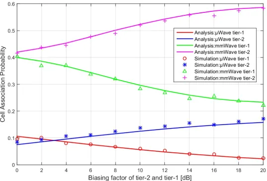
Figure 2 shows the cell association probability for a 2-tier mmWave and 2-tier μWave hybrid network as a function of the biasing factor of tier-2 and tier-1. The analytical results according to Lemma 1 and Lemma 2 are close to the simulation results. With the increasing biasing factor, the association probability for tier-2 in both mmWave and μWave network increases.
Figure 2. Cell association probability as a function of the biasing factor of tier-2 and tier 1 in dB
1 1 1
m
In Figure 3, we compare the analytical results for m
jP T and P Tj
with the simulation
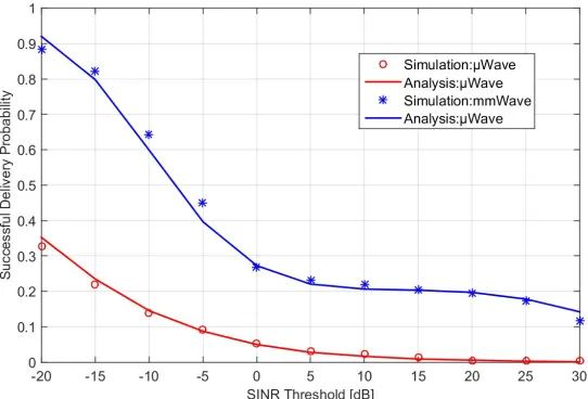
results in different SINR thresholds. It shows that our Proposition 1 and Proposition 2 approximate the simulation scenarios well. Unsurprisingly, the probability decreases with the increase of the SINR threshold. Considering the caching performance of the mmWave and μWave network separately, we calculate the successful delivery probability when the typical UE is already connected to the mmWave or μWave network for content j by
/ jj
P T , P Tjm
/ 1
j
,respectively. Figure 4 shows that with the increase of the SINR threshold the SDP decreases, but the performance of the mmWave network is much better than the μWave network which validates the accuracy of our association strategy. This is attributed to the employment of directional antennas. The mmWave network can be considered noise-limited and the antenna gain is high.
Figure 3. m
jP T , P Tj
and the overall SDP in varying SINR threshold for content j
1 1 2 2 1
m m
B B B B .
Figure 4. Successful delivery probability when the typical UE is already connected to the mmWave or μWave network for content j.
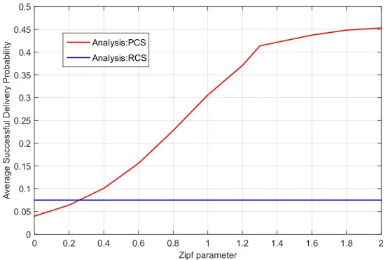
consisted of a 2-tier mmWave network and a 2-tier μWave network; for j51...100, the content isn’t cached in tier-2 of the mmWave and μWave network; for j100, all BSs don’t cache the content. Figure 5 shows that PCS performs much better than RCS with the Zipf parameter 0.8, and Figure 6 shows that with the increase of the Zipf parameter, the performance of PCS becomes much better than RCS. In Figure 6, when the Zipf parameter is small enough, the ASDP of PCS is smaller than RCS. This is because that the request probabilities of the contents become closer with the decrease of the Zipf parameter, and for PCS BSs cache the same contents which leads to the worse performance than RCS.
Figure 5. Average successful delivery probability of PCS and RCS for varying SINR threshold with Zipf parameter 0.8.
Figure 6. Average successful delivery probability of PCS and RCS for varying Zipf parameter with SINR threshold 0 dB.
5. Conclusions
association probability of the mmWave and μWave network, respectively. Also we theoretically analyze the ASDP as the caching performance metric. Finally, compared with Monte Carlo simulation results, our analytical model for the hybrid network performs quite well. Numerical results of ASDP for RCS and PCS show that PCS can achieve better performance in most situations.
Author Contributions: Shuyuan Zhao and Jihong Zhao modeled and analyzed the problem. Hua Qu and Gongye Ren proposed and implemented the result. Shuyuan Zhao wrote the paper.
Funding: This research was funded by National Natural Science Foundation of China (no.61531013) and National Science and Technology Major Project (no.2018ZX03001016).
Appendix A
Proof of Lemma 1:
If a typical UE is connected to the kth tier mmWave network , the averaged BRP for the kth
tier mmWave network is larger than others. Therefore,
1 1 , , 1 1 1, ( ) 0 1, ( ) 1,max
exp
0,
m km m m m
m k k k k k j j k j j j j
K
m m m m
k k k k j j j j
j j k
m m
K a
j j j
j m m k L k k
j j k k k k
K b
j j j
j k
j j k k k k
P G B L
P G B L
P G B L
P G B L
P G B
L
l f
l dl
P G B
P G B
l
P G B
0 0 10,
exp
0,
0,
exp
0,
k k k k k
K
j j j
k k j k k
j k k k
l
l
dl
P G B
l
l
dl
P G B
,(25)where ( )a follows the law of total probability and ( )b is from the definition of CCDF and PDF of the path loss given in (4) and (6). From the definition of the path loss PDF fLk( )x , we can see when
0
N kd
N kD
x L R , fLk( )=0x , which means the link between the typical UE and BS is in outage state.
Therefore, the expression derived above is the probability that a typical UE is connected to the kth
tier mmWave network.
Appendix B
Proof of Lemma 2:
Since UEs are offloaded to the μWave network only when the mmWave connection is not able to be established, and the BRP of the kth tier μWave network is
0( )
k k k
P L r B, the probability
,k
that a typical UE is connected to the kth tier μWave network can be given by:
, 0 , 0
2 0 0 1 1, 1/ 2 1 1,
= ( ) max ( )
exp ( ) ( )
exp
m
m
k k k k j j k j j j
K K
m
i iD k k k j j j
i j j k
K K
j j
m
i iD j k
i j j k k k
P L r B P L r B
R P L r B P L r B
P B
R r r
P B
2
1/0
1 1,
exp ( )
m k K K j j m
i iD j r
i j j k k k
P B
R r r f r dr
P B
. (26)
Using the fact that the null probability of a 2-D Poisson process with density in an area A is
exp(A), we can get:
1/ 2/
2
=exp
j j j j
j j
k k k k
P B P B
r r r
P B P B
, (27)
2
1
( ) 2 exp
k
k
r k k
d r r
f r r r
dr
. (28)
Combining the expressions derived above, we obtain
1/ 2 , 0 1 1, 2/2 2 2
0
1, 1
2 1
= exp ( )
= exp 2 exp exp
exp 2 exp
m k m m K K j j m
k i iD j r
i j j k k k
K K
j j
m
i iD k k j
j j k
i k k
K
m
i iD k
i
P B
R r r f r dr
P B
P B
R r r r dr
P B R
2/ 2 0 1 2/ 2 2/ 1 1 exp m K j j jj k k
K
k k k
m
i iD K
i j j j
j P B r rdr P B P B R P B
. (29)
Appendix C
Proof of Lemma 3:
The PDF frj k, ( )x can be derived according to (28):
, , 1 ( )= j k j k rd r x
f x
dx
, (30)
where
,
, ,
, 0 , , 0 , , 1/ , 1, , 2/ ( ) , 2 , , = ,
, ( ) max ( )
1 ( )
2
exp
j k
j k j k
j k k j k k l l k l j l l
j k
K
j j
j l r
j x
l l k
k k k
a
k j k l l
l j l
j
l
k k k
R x r x n k
r x P L r B P L r B
P B
r x f x dx
P B P B x P B
1 K x xdx
, (31)
where ( )a is obtained by (28) and (29) with a thinning homogeneous PPP jk of density jk.
Substituting (31) into (30), we obtain this lemma.
Appendix D
Proof of Proposition 1:
Assuming all biasing factors are 1, the coverage probability of the kth tier mmWave network
1 1 , , 1 1 1 11 2 ,
1 , , ,
1 \ 2
,
= SINR max
( ) = max ( ) m m m m l K
m m m m m m
j j k k k k k j j k j j j j
k
m m
K
m m m m
k k k k
k k k k j j j j
K m m j j k
k l l l i l i m k
l i o
m k
k m m k
k k
P T T P G B L P G B L
P G h L r
T P G B L P G B L
P G h L r
TL h P G
1 1 , 1 1 ( ) 2 , 0 1, 2 , max expexp 0, exp 0,
m m
k
K K
m m m m
l k k k k j j k j j j j
k l m K a j j k
m k j k L k k
m m
j j k
k k k k
j j
k
m k k k j k
m
k k
k k
I P G B L P G B L
P G Tl
L l f l dl
P G P G
P G Tl l l P G P G
0 1 K k j dl
, (32)
where ( )a follows the assumption that the mmWave network is noise-limited and under Rayleigh fading, m exp(1)
k
h . So, by combining (24) and (32), the expression of m
jP T given in Proposition 1 is obtained.
Appendix E
Proof of Proposition 2:
, , , ,, 0 ,
2 1 0 ( ) 2 1 0 ( ) 1 0
SINR = SINR ( )
/ ( )
exp / ( )
/ ( )
j k
j k
l j k
l j k
j k j k R
K
k l l k R
a K
I l l k R
b K
I k R
l
T r T f r dr
h Tr I P f r dr
Tr I P f r dr
Tr P f r dr
, (33)
where ( )a follows hk exp(1)
, and ( )b follows the assumption that the μWave network is
interference-limited. The interferences to the typical UE from the lth tier can be divided into two
groups: the interference Ilj
from the BSs caching content j and the interference
lj
I from the BSs
not caching content j. So the locations of interfering BSs can be modeled as two thinned PPPs of density l j l, and
1 j l,
l
, respectively. The Laplace transform lj
I
and lj
I
can be derived according to [19, eq. (37) and (38), Appendix C]:
2/ 2
,
/ = exp ,
lj
l
k l j l
I
k
P
Tr P r H T
P
, (34)
2/ 2
,
/ = exp 1 ,
lj
l
k l j l
I
k
P
Tr P r D T
P
, (35)
where
2 12 2 2
, 1,1 ;2 ; 2
T
H T F T
and D T
,
2T B2 2,1 2
. Combining (16),
(31), (33), (34) and (35), we can obtain Proposition 2.
References
1. Summary, E. Cisco Visual Networking Index : Global Mobile Data Traffic Forecast Update , 2010 – 2015. 2015, 2010–2015, doi:10.1016/j.tics.2013.12.009.
3. Yong, S. K.; Chong, C. C. An overview of multigigabit wireless through millimeter wave technology: Potentials and technical challenges. Eurasip J. Wirel. Commun. Netw. 2007, 2007, doi:10.1155/2007/78907.
4. Pi, Z.; Khan, F. An introduction to millimeter-wave mobile broadband systems. IEEE Commun. Mag.2011, 49, 101–107, doi:10.1109/MCOM.2011.5783993.
5. Akoum, S.; El Ayach, O.; Heath, R. W. Coverage and capacity in mmWave cellular systems. Conf. Rec. - Asilomar Conf. Signals, Syst. Comput.2012, 688–692, doi:10.1109/ACSSC.2012.6489099. 6. Jung, H.; Lee, I. H. Performance analysis of millimeter-wave multi-hop machine-to-machine networks based on hop distance statistics. Sensors (Switzerland)2018, 18, doi:10.3390/s18010204. 7. Ayach, O. El; Rajagopal, S.; Abu-Surra, S.; Pi, Z.; Heath, R. W. Spatially sparse precoding in millimeter wave MIMO systems. IEEE Trans. Wirel. Commun. 2014, 13, 1499–1513, doi:10.1109/TWC.2014.011714.130846.
8. Zhang, Z.; Chen, Y. Position fingerprint-based beam selection in millimeterwave heterogeneous networks. Sensors (Switzerland)2017, 17, doi:10.3390/s17092009.
9. Kulkarni, M. N.; Singh, S.; Andrews, J. G. Coverage and rate trends in dense urban mmWave cellular networks. 2014 IEEE Glob. Commun. Conf. GLOBECOM 2014 2014, 3809–3814, doi:10.1109/GLOCOM.2014.7037401.
10. Akdeniz, M. R.; Liu, Y.; Samimi, M. K.; Sun, S.; Rangan, S.; Rappaport, T. S.; Erkip, E. Millimeter wave channel modeling and cellular capacity evaluation. IEEE J. Sel. Areas Commun.2014, 32, 1164–1179, doi:10.1109/JSAC.2014.2328154.
11. Di Renzo, M. Stochastic Geometry Modeling and Analysis of Multi-Tier Millimeter Wave Cellular Networks. IEEE Trans. Wirel. Commun. 2015, 14, 5038–5057, doi:10.1109/TWC.2015.2431689.
12. Alejos, A. V.; Sanchez, M. G.; Cuinas, I. Measurement and analysis of propagation mechanisms at 40 GHz: Viability of site shielding forced by obstacles. IEEE Trans. Veh. Technol. 2008, 57, 3369–3380, doi:10.1109/TVT.2008.920052.
13. Bai, T.; Heath, R. W. Coverage and Rate Analysis for Millimeter Wave Cellular Networks. 2014, 14, 1100–1114, doi:10.1109/TWC.2014.2364267.
14. Turgut, E.; Cenk Gursoy, M. Coverage in Heterogeneous Downlink Millimeter Wave Cellular Networks. IEEE Trans. Commun.2017, 65, 4463–4477, doi:10.1109/TCOMM.2017.2705692. 15. Elshaer, H.; Kulkarni, M. N.; Boccardi, F.; Andrews, J. G.; Dohler, M. Downlink and uplink cell
association with traditional macrocells and millimeter wave small cells. IEEE Trans. Wirel. Commun.2016, 15, 6244–6258, doi:10.1109/TWC.2016.2582152.
16. Vuppala, S.; Biswas, S.; Ratnarajah, T. An Analysis on Secure Communication in Millimeter/Micro-Wave Hybrid Networks. IEEE Trans. Commun. 2016, 64, 3507–3519, doi:10.1109/TCOMM.2016.2587287.
17. Woo, S.; Jeong, E.; Park, S.; Lee, J.; Ihm, S.; Park, K. Comparison of caching strategies in modern cellular backhaul networks. Proceeding 11th Annu. Int. Conf. Mob. Syst. Appl. Serv. - MobiSys ’13 2013, 319, doi:10.1145/2462456.2464442.
18. Tamoor-ul-Hassan, S.; Bennis, M.; Nardelli, P. H. J.; Latva-Aho, M. Modeling and Analysis of Content Caching in Wireless Small Cell Networks. 2015, 1–5, doi:10.1109/ISWCS.2015.7454454. 19. Li, K.; Yang, C.; Chen, Z.; Tao, M. Optimization and Analysis of Probabilistic Caching in N-Tier
Heterogeneous Networks. IEEE Trans. Wirel. Commun. 2018, 17, 1283–1297, doi:10.1109/TWC.2017.2777483.
20. Bastug, E.; Bennis, M.; Debbah, M. Living on the edge: The role of proactive caching in 5G wireless networks. IEEE Commun. Mag.2014, 52, 82–89, doi:10.1109/MCOM.2014.6871674. 21. Wang, X.; Chen, M.; Taleb, T.; Ksentini, A.; Leung, V. C. M. Cache in the air: Exploiting content
caching and delivery techniques for 5G systems. IEEE Commun. Mag. 2014, 52, 131–139, doi:10.1109/MCOM.2014.6736753.
23. Tamoor-ul-Hassan, S.; Bennis, M.; Nardelli, P. H. J.; Latva-aho, M. Caching in Wireless Small Cell Networks: A Storage-Bandwidth Tradeoff. IEEE Commun. Lett. 2016, 20, 1175–1178, doi:10.1109/LCOMM.2016.2543698.
24. Bastug, E.; Bennis, M.; Debbah, M. Cache-enabled small cell networks: Modeling and tradeoffs. In 2014 11th International Symposium on Wireless Communications Systems (ISWCS); IEEE, 2014; pp. 649–653.
25. Chae, S. H.; Choi, W. Caching Placement in Stochastic Wireless Caching Helper Networks: Channel Selection Diversity via Caching. In IEEE Transactions on Wireless Communications; 2016; Vol. 15.
26. Liu, D.; Yang, C. Caching Policy Toward Maximal Success Probability and Area Spectral Efficiency of Cache-Enabled HetNets. IEEE Trans. Commun. 2017, 65, 2699–2714, doi:10.1109/TCOMM.2017.2680447.
27. Yang, C.; Yao, Y.; Chen, Z.; Xia, B. Analysis on Cache-Enabled Wireless Heterogeneous Networks. IEEE Trans. Wirel. Commun.2016, 15, 131–145, doi:10.1109/TWC.2015.2468220. 28. Lu, W.; Di Renzo, M. Stochastic Geometry Modeling of Cellular Networks: Analysis, Simulation
and Experimental Validation. 2015, doi:10.1145/2811587.2811597.
29. Haenggi, M.; Ganti, R. K. Interference in Large Wireless Networks; 2008; Vol. 3; ISBN 1300000015. 30. Hunter, A.; Andrews, J.; Weber, S. Transmission capacity of ad hoc networks with spatial
diversity. IEEE Trans. Wirel. Commun.2008, 7, 5058–5071, doi:10.1109/T-WC.2008.071047. 31. Ding, M.; Wang, P.; Member, S.; David, L. Performance Impact of LoS and NLoS Transmissions
in Small Cell Networks. 2015, 1276, 1–30, doi:10.1109/TWC.2015.2503391.
32. Blaszczyszyn, B.; Karray, M. K.; Keeler, H. P. Using Poisson processes to model lattice cellular networks. Proc. - IEEE INFOCOM2013, 773–781, doi:10.1109/INFCOM.2013.6566864.
33. Rangan, S.; Rappaport, T. S.; Erkip, E. Millimeter Wave Cellular Wireless Networks: Potentials and Challenges. 2014, 1–17, doi:10.1109/JPROC.2014.2299397.
34. Jo, H. S.; Sang, Y. J.; Xia, P.; Andrews, J. G. Heterogeneous cellular networks with flexible cell association: A comprehensive downlink SINR analysis. IEEE Trans. Wirel. Commun. 2012, 11, 3484–3494, doi:10.1109/TWC.2012.081612.111361.