KNN-DTW Based Missing Value Imputation for
Microarray Time Series Data
Hui-Huang Hsu, Andy C. Yang, Ming-Da Lu Department of Computer Science & Information Engineering,
Taipei, Taiwan, R.O.C.
Email: [email protected], [email protected]
Abstract—Microarray technology provides an opportunity
for scientists to analyze thousands of gene expression profiles simultaneously. However, microarray gene expression data often contain multiple missing expression values due to many reasons. Effective methods for missing value imputation in gene expression data are needed since many algorithms for gene analysis require a complete matrix of gene array values. Several algorithms are proposed to handle this problem, but they have various limitations. In this paper, we develop a novel method to impute missing values in microarray time-series data combining k-nearest neighbor (KNN) and dynamic time warping (DTW). We also analyze and implement several variants of DTW to further improve the efficiency and accuracy of our method. Experimental results show that our method is more accurate compared with existing missing value imputation methods on real microarray time series datasets.
Index Terms—microarray time series data, missing value
imputation, dynamic time warping, k-nearest neighbor.
I. INTRODUCTION
Recently, microarray technology has become one of the important tools in biological researches. Microarray makes it possible to monitor thousands of gene expressions in a single experiment. Numerous gene expression data can be generated simultaneously via this high throughput biological technology. Microarray time-series data are generated by using cDNA microarray technology. It was previously found in many studies that gene expression values represent the reaction of each gene after the hybridization effect across time [1,2]. Each gene expression value represents different reaction degrees resulted from experiments. These quantitative values are in the format of logarithm. This kind of data provides a possible means for the inference of transcriptional regulatory relationships among the genes on the microarray gene chips. The discovery of specific gene pairs with highly-correlated relations could provide valuable information for biologists to predict important biological reactions [3].
Nevertheless, microarray gene expression data usually contain multiple missing values. A specific portion of gene expression values that do not exist in microarray gene expression raw data are called missing values. For subsequent analysis of microarray gene expression data, these kind of missing values need to be effectively estimated and imputed. The reason why missing values
occur may result from experimental operations, experimental inaccuracy, or unobvious reaction at that time slot of certain genes [4]. If there is a particular gene I with one missing value at time slot J, then YIJ is denoted to represent the target missing value.
In this paper, we propose a novel approach combining k-nearest neighbor (KNN) and dynamic time warping (DTW) to impute missing values in DNA gene expression microarray time series raw datasets. Furthermore, we also survey and analyze several techniques for accuracy and efficiency refinements of the DTW algorithm to further improve our method. Compared with existing imputation methods, our method is more effective because we not only keep the advantage of the KNN method but also make improvements on it to reach a better result. Our method can impute missing values efficiently in spite of the existence of outliers and time delays. Moreover, our method takes DTW as the similarity measurement of two genes so that it is still practical while handling gene sequences of different lengths. Experimental results show that the proposed method with specific variants of DTW outperforms others in imputing missing values in microarray time series data. The remaining of this paper is organized as follows. In Section II, discussions on existing imputation methods for missing values in microarray time-series dataset are given. The proposed method is delineated in detail in Section III. Section IV described the involved datasets and the estimation of imputation accuracy. The experimental result is then presented and discussed in Section V. The concluding remarks are drawn in Section VI along with future work.
II. LITERATURE REVIEW
sequential k-nearest neighbor (SKNN) method [6]. The method imputes the missing values sequentially from the genes with least missing values, and uses the imputed values for the later imputation. This study is typically an example showing the effectiveness of KNN with some improvements on it. Besides KNN or KNN-based imputation methods, there are still other works proposing several methods of different aspects. Oba et al. propose an estimation method for missing values based on Bayesian principal component analysis (BPCA) [7]. The method combines mathematical theorems and needs no modelling parameters which are difficult to determine. The results outperform the KNN and SVD imputations according to the authors’ evaluations. Moreover, an imputation method called LLS-impute based on the local least squares formulation is proposed to estimate missing values in the gene expression data [8].
For existing imputation methods, BPCA is shown to outperform others. However, it is not easy to decide the number of principal axes while applying BPCA for missing value imputation [9]. Existing methods for microarray missing value imputation mainly utilize k-nearest neighbor (KNN) or KNN-like approaches to estimate the missing values. When applying KNN to impute missing values in microarray time series-data, we have to choose a number of k similar genes without missing entries at the same time slot (experiment) as the target missing value. Besides, we still need to estimate how similar the two genes of interest are to identify whether the two genes have regulatory relations. However, most of the similarity measurements take the statistical or mathematical correlations among genes into consideration. These principles may be unsuitable to the microarray time-series data because of the existence of outliers. Outliers influence much on the correlation coefficient measurements, especially when there are two or more outliers occurring in the time-series data set. A study suggests that outliers do exist in certain microarray datasets [10]. Also, when identifying similarity of two genes in microarray time-series data, comparing local similarity is usually more important than comparing all time slot points. The reason is that even genes with known regulations may have reaction delay or offsets among time axis in microarray experiment results [11]. As a result, it is necessary to apply a similarity measurement method that has the capability of pointing out local similarity and is also effective even with certain existing outliers in microarray time-series data.
III. METHOD
To overcome the difficulty mentioned above and to achieve better imputation results, we propose a novel missing value imputation method based on KNN and dynamic time warping (DTW). With our method, local similarity and shifted trends of gene expression data between each gene pair can be discovered. Studies argue that it is more important to observe and find out whether there exist sub-sequences with highly similar relations when analyzing whole microarray time series data. However, most of existing studies and approaches take
Euclidean distance that identifies global similarity into account as the measurement to determine whether two genes are similar or not. Also, DTW is practical even though the two gene sequences to be aligned are of different length, where this often happens in real microarray dataset. Besides, offsets among time-axis do not influence much on DTW because DTW generates corresponding mappings of two sequences according to their similar shapes. Outliers will not influence on DTW critically compared with Euclidean distance or Pearson correlation coefficients. With our method, better imputation results can hence be achieved. Moreover, we also try our method with several variants of DTW to further improve its efficiency and accuracy of imputation. This section briefly describes the KNN method and the DTW algorithm, followed by the combined method for missing value imputation.
A. K-Nearest Neighbor Imputation Method
The k-nearest neighbor (KNN) method selects genes with expression values similar to those genes of interest to impute missing values. For example, if we consider gene G that has one missing values at experiment time slot T, KNN would find K other genes that have a value at experiment time slot T, but with expression values most similar to Gene G in experiments time slot points except for T. A weighted average of values at experiment time slot T from the chosen K closest genes is then used as estimation for the missing value in gene G. As for the weighted average, the weighted value of each gene in the K closest similar genes is given by the similarity of its expression to that of gene G. To determine the k closest genes which are similar to the target gene G with missing values to impute, matrices such as Euclidean distance measurement, Pearson correlation coefficient, or other distance-based similarity measurements are applied. Usually, Euclidean distance measurement is the most commonly used metric for this purpose. The steps of KNN imputation are as follows:
Step1. In order to impute the missing value GIJ for
gene I at time slot J, the KNN-impute algorithm chooses k genes that are most similar to the gene I and with the values in position k not missing.
Step2. If Euclidean distance measurement is employed for two gene expression vectors gx = <ex1, ex2, ex3…exn>
and gy = <ey1, ey2, ey3…eyn>, the Euclidean distance
between gx and gy can be calculated as follows:
dis(gx, gy) =
nt
t y t
x
e
e
1
2 ,
,
)
(
(1)
Step3. The missing value is estimated as the weighted average of the corresponding entries, in the selected k expression vectors:
GIJ = iJ (2) k
i
i
e
W
1
)
,
(
1
* i ig
g
dis
W
(3),where (4)
k i ig
g
dis
1 *)]
,
(
/(
1
[
and g* denotes the set of k genes closest to gi
When applying the KNN-based method for the imputation of missing values, there are no constant criteria for selecting the best k-value and similarity measurements. Both k-value and similarity measurements have to be determined empirically. It is not constant for determining the k value. Choosing a small k value produces poorer performance after imputation. On the contrary, choosing a large neighbourhood may include instances that are significantly different from those containing missing values. However, on study shows that setting k-value between 10 and 20 brings the best results for KNN imputation [5]. With this result, KNN can be an effective and intuitive imputation method if it works with a proper similarity measurement for genes.
B. Dynamic Time Warping
Dynamic time warping (DTW) is a commonly-used algorithm in voice and pattern recognition [12,13]. It has been shown that DTW performs well to find out the similarity for a pair of time series data [14,15]. In this paper, we combine the KNN method with the DTW algorithm as the similarity measurement to estimate the missing value in microarray time-series data. In general, the dynamic time warping (DTW) method is used to warp and match generic sequences of numbers that can be viewed as curves in a proper coordinate system. The aim of DTW is to obtain a precise matching along the temporal axis, and to maximize the number of point-wise matches between two time series. The alignment of temporal patterns by DTW has traditionally been used in the recognition of speech signals. This method is a widely-used algorithm for string comparison and for the alignment of time series data. If two series with time points are given as input, the DTW algorithm can select the best possible alignment between them by minimizing a local distance between the series points.
DTW is a recursive algorithm that matches each two-point pair from the first element to the last element on input sequences. After the table recording all local optimal paths and corresponding points is completed, a multiple of its last computed value returns the DTW distance between the two sequences. If we are going to align two sequences that are similar with observation, the application of Euclidean distance or Pearson correlation coefficient of these two sequences may have poor performance due to shifts on time axis. With DTW mapping method, local similarity can be found as the best path within the two comparison sequences. As a result, if two genes with similar gene expression values at certain parts in microarray time series data are analyzed by DTW, it is more precise for similarity measurement because DTW can discover their similarity that cannot be
identified with other similarity measurements. Equations of DTW algorithm are as follows:
Distance of two time slot pints:
The distance between the elements of the two time series is computed as:
i
i
y
x
j
i
dis
(
,
)
(5)
Base Conditions:
e(0,0) = 0;
e(1,1) = dis(x1,y1)*WD;
e(i,0) = ∞ for 1≦ i ≦ I;
e(0,j) = ∞ for 1≦ j ≦ J; (6) where WD is the weighted value for the paths in the
diagonal direction. Recursive Relation:
H j i D j i V j iW
y
x
dis
j
i
e
W
y
x
dis
j
i
e
W
y
x
dis
j
i
e
j
i
e
*
)
,
(
)
,
1
(
*
)
,
(
)
1
,
1
(
*
)
,
(
)
1
,
(
min
)
,
(
(7) where Wv, WD, and WH denote the weighted value forthe paths in the vertical, diagonal, and horizontal directions respectively.
Output: DTW distance for two sequences X and Y:
DTW(X,Y) =
)
,
(
1
j
i
e
m
n
(8)where length of X and Y are n and m respectively.
C. Imputation Method Combining KNN and DTW
While handling missing value imputation problems, we combine the KNN method with the DTW algorithm. DTW is utilized as the similarity measurement between gene expression values at time slots. The combined method substitutes equation (9) and equation (10) for equation (3) and equation (4) respectively.
)
,
(
1
* i ig
g
DTW
W
(9) where (10)
k i ig
g
DTW
1 *)]
,
(
/(
1
[
Missing values for the target gene are hence imputed with our proposed method.
D. Refinement of the Algorithm
1) Computational Efficiency
The critical disadvantage of DTW is its high computational cost. The time complexity of the traditional DTW algorithm is O(n*m) for two input sequences with length n and m, respectively. Despite the high throughput and computational ability of modern computers, speeding up the calculations for DTW distance is still essential when the size of involved data is very large. As we will show in Section IV, we use the Spellman’s dataset to perform missing value imputation with totally 6178 genes in the dataset. However, if we naively use the original DTW algorithm to calculate DTW distance of the total 6178 genes, the calculation time needed is awfully amazing and reduces the practicability of the algorithm. As a result, several methods to speed up the calculation of DTW are proposed. Among all existing methods, we find the most useful one proposed in [16]. The authors propose an approximation of DTW called FastDTW that has linear time and space complexity. In other words, if there are two time series sequences with near the same length n, time complexity for FastDTW is only O(n). The method uses a multilevel approach that recursively projects a solution from a coarse resolution version of original data and refines the projected solution. With FastDTW, the computational cost can hence be reduced. FastDTW works somehow like the “divide and conquer” technique in the algorithm field. It uses a multilevel approach with three operations:
a) Coarsening: Coarsening means that FastDTW
shrinks a time series into a smaller one which represents the same curve as accurately as possible with fewer data points.
b) Projection: After FastDTW performs the
coarsening step, it will find a minimum- distance warping path at a lower resolution, and use the path to guess another minimum-distance warping path in a higher resolution.
c) Refinement: Finally, FastDTW refines each
warping path in every resolution projected from a lower resolution with local adjustments.
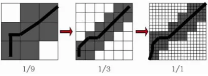
FastDTW cut the points needed from original time series to the lowest resolution from 1/1 to 1/2 to 1/4 and so forth, and then projects paths from each lower resolution to a higher one. For example, if there are 18 points in an original time series, FastDTW cuts the points needed from 18 with a two-times reducing rate. This forms every resolution in the coarsening process. However, according to our testing, we find that coarsening with a three-times reducing rate performs better than coarsening with a two-times reducing rate in terms of the dataset involved. This is because the dataset we use only contain 18 or 17 time points and only need two times of coarsening. As a result, we modify the FastDTW algorithm and set the coarsening rate from 1/1 to 1/3 to 1/9 as shown in Fig. 1. With three-times reducing rate, we can retrieve better computational efficiency with almost the same accuracy. Finally, FastDTW gives a specific tolerance region for projecting
the warping path from a lower resolution to increase the probability that paths of FastDTW runs through paths of real DTW. This procedure is performed to slightly improve the accuracy of FastDTW.
2) Accuracy of imputation
The other attractive issue for the improvement of the DTW algorithm is in accuracy increasing. Although DTW has been used in various fields with success, there is still a drawback called the singularity problem [17]. In some cases, DTW would lead to unintuitive alignments where a single point on one time series is mapped onto a large subsection of the other time series. In other words, a specific point on one input sequence may map into even more than three points on the other sequence. This kind of undesirable behavior is so called the singularity problem. As we mentioned in previous sections, DTW works well due to its capability of discovering local similarity of two sequences so that forms a dynamic mapping which is better than usual global similarity measurement like Euclidean distance or Pearson correlation coefficient. However, when the two sequences to be aligned are highly similar but with only slightly different height of the peaks mapped on the two sequences, DTW will perform a one-to-many mapping. This reduces the effectiveness of the algorithm because this kind of mapping is not expectative theoretically and will easily fail to find obvious and intuitive alignments for sequences. As a result, modifications on DTW to mitigate the singularity problem are essential.
Figure 1. Modification of FastDTW
Several works to mitigate this problem are developed with certain effectiveness respectively. We survey and analyze existing methods aiming to reduce the singularity problem and choose four of them to implement on our proposed missing value imputation method. Within the four methods, three of them are typical constraining modifications of DTW developed one decade ago, while the other one is a recently-revised method. In the following paragraph, we give a brief description on the four methods.
a) Windowing: Berndt and Clifford proposed a
b) Slope weighting: Kruskall and Liberman
proposed a modification of DTW so that the recursive equation in the original DTW algorithm is replaced by r(i,j) = d(i,j) +min{r(i-1,j-1) , X*r(i-1, j), X*r(i, j-1)} where X is a positive real number [19]. With this constraint, the warping path is biased toward the diagonal if the weighted value X gets larger. Since each step in recursive procedures of DTW searches for minimum distance summed up so far, the warping path with slope weighting tends to walk through the diagonal direction if larger weighted value X is assigned. This modification of DTW takes the weighted value into consideration that it tries to slightly encourage the warping path goes in diagonal direction to reduce singularity.
c) Step patterns (Slope constraint): Itakura
proposed a permissible step for the warping path with r(i,j) = d(i,j)+min{r(i-1,j-1) , r(i-1, j-2), r(i-2,j-1)}[20]. With this constraint, the warping path is forced to move one diagonal step for each step parallel to an axis. In other words, if the DTW algorithm selects the horizontal or vertical adjacent path in one step, the subsequent path is forced to move one diagonal step.
d) Derivative Dynamic Time Warping: Keogh and
Pazzani introduced a modification of DTW [21]. This modification of DTW is called derivative dynamic time warping (DDTW). The author considered only the estimated local derivatives of gene expression values in sequences instead of using the whole gene expression values themselves. DDTW uses a modified estimation to substitute for equation (5) while calculating the distance between two time points from two time series. This estimation equation is as follows:
Distance for two time points in two sequences
dis(i, j) = | E(Xi) – E(Yi)|2 while
E(Xi) ={ (Xi – Xi-1) + [(Xi+1 – Xi-1) / 2] } / 2 , and
E(Yi) ={ (Yi – Yi-1) + [(Yi+1 – Yi-1) / 2] } / 2 (11)
DDTW takes moving trends of certain subsequences into account in order to judge the similarity of the two sequences. Instead of the distance between two points, DDTW is said to be more sensitive to discover local similarity of two sequences.
Among four above-mentioned methods, windowing and slope weighting are intuitive because they simply form the constraints to force the warping path not to go along the horizontal or vertical direction too much. Step patterns also try to mitigate the singularity problem by leading the warping path to cross the diagonal if the previous step goes along the X-axis or Y-axis. DDTW seems to work well on certain datasets, but it is not suitable for some cases such as sequences with great portions of empty values. The four variants of the DTW algorithm may successfully mitigate the singularity problem under specific situations.
For the four variants of DTW mentioned above, we consider that slope weighting should bring the best results for imputation. This is because slope weighting is more flexible that slightly encourages the warping path goes to the diagonal. For the microarray dataset we use, what
counts lies in local similarity of two genes. Forcing the warping path to go to the diagonal too much may mitigate the singularity problem, but it is also at the risk of losing the alignment that reveals the best mapping of two genes. Slope windowing will be effective if the window size w is small. On the other hand, imputation will be brittle as the window size w is set to be too large. Step patterns also forces the warping path with its constraints. This may results in possible loss of the best mapping. DDTW is not suitable for our microarray time series dataset. The reason is because of the great portion of missing values. Our goal is to retrieve the most proper modification of DTW so that our proposed imputation method can acquire the best results. To fit this need, we have implemented the four above modifications for DTW on our proposed method. We also compare the imputation effectiveness resulted from of these modifications of DTW in order to improve the accuracy of our proposed method. Experimental results stand by our assumptions that performing windowing and slope weighting brings a better result. The detail will be presented and discussed in Section V.
IV.DATASETS AND PERFORMANCE ASSESSMENT
In order to evaluate the effectiveness of the proposed imputation method, we implement the method on real microarray datasets. In this section, we first give a brief description about the dataset involved in our experiments. Subsequently, performance measurement of imputation methods is explained. The NRMS equation is used to assess whether the imputation method are effective or not.
A. Real Microarray Dataset
Spellman et al. and Cho et al. provided the yeast
microarray dataset (
B. Assessment of Imputation Accuracy
After the imputation for missing values, we have to assess the performance of our method and the comparison with existing imputation methods. For assessment of imputation accuracy, genes with missing values in microarray gene expression data are first filtered to generate a complete matrix. As for Spellman’s dataset, there are about 4304 genes in the complete matrix. Missing values with different missing rates ranging from 1%, 5%, 10%, 15% and 20% of the data in the complete matrix are deleted at random to create testing datasets. Afterward, we impute missing values in testing datasets with our method to recover the introduced missing values for each data set. The estimated values are compared to those in the complete matrix. The commonest way for the assessment of missing value imputation is to calculate the normalized root mean square (NRMS) error. The most commonly-used equation for NRMS error is as follows:
NRMS=
]
[
]
)
[(
y
predicty
known 2std
y
knownmean
(12)
where and are estimated values
and known values in the complete matrix, respectively,
and is the standard deviation of known values. After generating complete matrices and randomly-removed testing datasets, we will impute missing values with our method. NRMS errors will also be calculated as the assessment to be compared with those of other imputation methods.
predict
y
]
[
y
knownknown
y
std
V.EXPERIMENTAL RESULTS
A. Mission Value Imputation
We combine the KNN method and the modified DTW algorithm based on FastDTW, along with four variants of DTW to impute missing values in alpha and cdc28 testing datasets. NRMS errors are then calculated as the assessment to determine whether an imputation method is effective or not. An imputation method is said to outperform other methods if and only if its NRMS value is lower than that of others. We first implement our method by using FastDTW-based DTW algorithm. Then we also experiment on the four variants of DTW for accuracy improvement. Moreover, we add the original KNN imputation method, zero imputation, row average imputation, BPCA imputation and LLS imputation in our experiment. We try to compare and explain imputation results from all mentioned methods. Imputations are performed on alpha sub-dataset and cdc28 sub-dataset in Spellman’s yeast microarray datasets. Missing rates range from 1%, 5%, 10%, 15%, to 20% individually. The number of K for KNN is set from 10, 15, 20, 50, and 100. DTW with weighting value ranges from 1.2 to 1.8 because we find that the effectiveness is reduced if the weighting value is larger than 1.8. DTW with windowing parameter ranges from 2 to 5 for the same reason. For
each experiment, we run 10 times and calculate the average value to reduce the randomness. We then pick out parameters that generate the best result for each method and compare the NRMS values among these methods.
B. Results and Discussion
With the experimental results, we find that the most proper parameter for each variant of DTW differs. For observation convenience, here we merely list the result of each method generated with the parameter that brings the best outcome. We observe and compare the results above and hence make some summaries. First, for all experimental results, we find that methods relative to KNN including KNN, FastDTW, and FastDTW with variants of DTW retrieve the best results when the number of K is set between K =10 and K = 20. This stands for Troyanskaya’s research in 2001. As a result, while applying KNN or KNN-like methods to impute missing values in microarray time series data, setting the number of K between 10 and 20 generates the best result empirically. Assigning the value of K less than 10 or more than 20 will not bring a better result.
Besides, we find that the best result occurs when we apply our proposed method with FastDTW-based modification and slope weighting with weighted value between 1.5 and 1.8. For cdc28 sub-dataset, FastDTW with windowing and slope weighting both surpass other imputation methods. This indicates that DTW works well with slightly weighted value that forces the warping path to the diagonal direction. But if we put too much force, it will generate unfavorable results. As for the various missing rate of experimental dataset, we find that our proposed method with FastDTW-based modification works better than the traditional KNN imputation method in most cases. Moreover, if we add proper variants such as slope weighting with weighted value between 1.5 and 1.8, or windowing with window size = 2 for the improvement of DTW, it will bring better results. The proposed DTW imputation method outperforms other methods including BPCA, especially when the missing rate is large such as 15% or 20%.
performing windowing and slope weighting improves the accuracy of the proposed method. In order to reduce the problem of singularity, several techniques are proposed.
As shown in Fig. 2, average imputation and zero imputation seem to be brittle. These two simple imputation methods provide limited help. The imputation method that only utilizes KNN with FastDTW achieves better results than using KNN. This proves that taking DTW distance as the similarity measurement is more suitable than taking Euclidean distance while handling microarray time series data. However, if we modify the algorithm with step patterns or DDTW, the accuracy of imputation decreases. This shows that it is improper to apply step patterns and DDTW for the dataset. The reason is discussed in previous paragraph. BPCA and LLS seem to outperform KNN and other brittle imputation methods. Using FastDTW with windowing results in better results than LLS brings. The most effective method is using FastDTW with slope weighting
that slightly outperforms than BPCA. Sequences of effectiveness of these imputation methods may change a little bit in certain percentage of missed data. This may result from the randomness while deciding which values to be removed in the complete matrix.
Fig. 3 illustrates almost the same situation as Fig. 2. Basically results of all imputation methods are worsened a little. This is because the cdc28 sub-dataset contains more missing values than the alpha sub-dataset. Theoretically, NRMS error increases while missing values are getting more in the dataset. We can also see that using FastDTW with windowing and slope weighting both outperform BPCA. Furthermore, even using FastDTW brings better results than BPCA when the missing rate is larger than 15%. This shows the weakness of BPCA while dealing with microarray time series dataset with a large portion of missing values. To summarize, using our proposed method with the variant of slope weighting can retrieve the best imputation results.
Figure 2. Imputation results of alpha dataset
Figure 3. Imputation results of cdc28 dataset
VI.CONCLUSION
Missing value imputation is very important in microarray gene expression time series data. In this paper, we propose a novel method that combines the traditional KNN method with the DTW algorithm to perform the imputation. We also implement variants of DTW both
the imputation method. We believe our approach facilitates research for microarray gene expression data.
REFERENCES
[1] J. DeRisi, R. Iyer, and Brown P, “Exploring the metabolic and genetic control of gene expression on a genomic scale,” Science, vol.278, pp.680-686, 1997.
[2] P.T. Spellman, G. Sherlock, M.Q. Zhang, V.R. Iyer, K. Anders, M.B. Eisen, P.O. Brown, D. Botstein, and B. Futcher, “Comprehensive identification of cell cycle-regulated genes of the yeast saccharomyces cerevisiae by microarray hybridization,” Mol. Biol. Cell, vol.9, pp.3273-3297, 1998.
[3] D.S.V. Wong, F.K. Wong, and G.R. Wood, “A multi-stage approach to clustering and imputation of gene expression profiles,” Bioinformatics, vol.23, pp.998-1005, 2007.
[4] E. Acuna and C. Rodriguez, “The treatment of missing values and its effect in the classifier accuracy,” Classification, Clustering and Data Mining Applications, pp.639-648, 2004.
[5] O. Troyanskaya, M. Cantor, G. Sherlock, P. Brown, T. Hastie, R. Tibshirani, D. Botstein, and R.B. Altman, “Missing value estimation methods for DNA microarrays,” Bioinformatics, vol.17, pp.520-525, 2001. [6] H. Kim, G.H. Golub, and H. Park, “Imputation of missing
values in DNA microarray gene expression data,” in: Proc. of the IEEE Computational Syst. Bioinformatics. Conf., pp.572-573, 2004.
[7] S. Oba, M. Sato, I. Takemasa, M. Monden, K. Matsubara, and S. Ishii, “A Bayesian missing value estimation method for gene expression profile data,” Bioinformatics, vol.19, pp.2088-2096, 2003.
[8] H. Kim, G. H. Golub, and H. Park, “Missing value estimation for DNA microarray gene expression data: local least squares imputation,” Bioinformatics, vol.21, pp.187-198, 2005.
[9] X. Wang, A. Li, Z. Jiang, and H. Feng, “Missing value estimation for DNA microarray gene expression data by support vector regression imputation and orthogonal coding scheme,” BMC Bioinformatics, vol.7, pp.1-10, 2006.
[10]A.C. Yang, H.H. Hsu, and M.D. Lu, “Outlier filtering for identification of gene regulations in microarray time-series data,” in: Proc. of the 3rd Intl. Conf. on Complex, Intelligent and Software Intensive Syst., pp.854-859, 2009. [11]V.S. Tseng, L.C. Chen, and J.J. Chen, “Gene relation
discovery by mining similar subsequences in time-series microarray data,” in: Proc. of the IEEE Symposium on Computational Intelligence in Bioinformatics and Computational Biol., pp.106-112, 2007.
[12]C. Furlanello, S. Merler, and G. Jurman, “Combining feature selection and DTW for time-varying functional genomics,” IEEE Trans. on Sig. Processing, vol.54, pp.2436-2443, 2006.
[13]H.M. Yu, W.H. Tsai, and H.M. Wang, “Query-by-singing system for retrieving karaoke music,” IEEE Trans. on Multimedia, vol.10, pp.1626-1637, 2008.
[14]C. Myers, L. Rabiner, and A. Roseneberg, “Performance tradeoffs in dynamic time warping algorithms for isolated word recognition,” IEEE Trans. on Acoustics, Speech, and Signal Processing, vol.ASSP-28, pp.623-635, 1980.
[15]L. Rabiner, A. Rosenberg, and S. Levinson, “Considerations in dynamic time warping algorithms for discrete word recognition,” IEEE Trans. on Acoustics,
Speech, and Signal Processing, vol.ASSP-26, pp.575-582, 1978.
[16]S. Salvador and P. Chan, “Toward accurate dynamic time warping in linear time and space,” Intelligent Data Analysis, vol.11, pp.561-580, 2007.
[17]H. Sakoe and S. Chiba, “Dynamic programming algorithm optimization for spoken word recognition,” IEEE Trans. on Acoustics, Speech, and Signal Processing, vol.ASSP-26, pp.43-49, 1978.
[18]D. Berndt and J. Clifford, “Using dynamic time warping to find patterns in time Series,” in: Proc. of the Workshop on Knowledge Discovery in Databases, pp.359-370, 1994. [19]J.B. Kruskall and M. Liberman, “The symmetric time
warping algorithm: from continuous to discrete,” in: Time Warps, String Edits, and Macromolecules: The theory and Practice of String Comparison, 1983.
[20]F. Itakura, “Minimum prediction residual principle applied to speech recognition,” IEEE Trans. on Acoustics, Speech, and Signal Processing, vol.ASSP-23, pp.52-72, 1975. [21]E. Keogh and M. Pazzani, “Derivative dynamic time
warping,” in: Proc. of the 1st SIAM Intl. Conf. on Data Mining, pp.1-11, 2001.
[22]R. Cho, M. Campbell, E. Winzeler, L. Steinmetz, A. Conway, L. Wodicka, T. Wolfsberg, A. Gabrielian, D. Landsman, and D. Lockhart, “A genome-wide transcriptional analysis of the mitotic cell cycle,” Mol. Cell, vol.2, pp.65-73, 1998.
Hui-Huang Hsu is an associate professor of Computer Science and Information Engineering at Tamkang University, Taipei, Taiwan. He received his Ph.D. degree in electrical engineering from the University of Florida in 1994. His current research interests are in the areas of machine learning, data mining, bioinformatics, and multimedia processing. Dr. Hsu is a senior member of the IEEE
Chao-Hsun Yang has an alias of Andy C. Yang. He is a Ph.D. candidate in the Department of Computer Science and Information Engineering at Tamkang University, Taipei, Taiwan. He received his M.S. degree from the Department of Computer Science and Information Engineering at Tamkang University, Taiwan, R.O.C., in 2005. His research interests are in bioinformatics and computer algorithms.