To Study the Surface Properties of GFRP in USM
by using Taguchi Method
Raminder Singh Bhatia Ashwani Tayal
Department of Mechanical Engineering Department of Mechanical Engineering Sant Baba Bhag Singh Institute of Engineering & Technology
Padhiana dist. Jalandhar Rayat Bahra University Mohali, India
Abstract
USM has become an important and cost-effective method of machining extremely tough and brittle materials. It is widely used in the process of drilling and machining on sections of complex geometry and intricate shapes. The work piece material selected in this experiment is glass fiber reinforced plastic (GFRP) taking into account its wide usage in industrial applications. In today’s world GFRP contributes to almost one third of the world’s production and consumption for industrial purposes. This material is not used for traditional machining due to chipping or fracturing many similar problems can be successfully solved using ultrasonic technologies. The input variable parameters are type of tool material, frequency, amplitude, and concentration in USM. Taguchi method is applied to create an L18 orthogonal array of input variables using the Design of Experiments (DOE). The effect of the variable parameters mentioned above upon machining characteristics such as Material Removal Rate (MRR) and Surface Roughness (SR) and tool wear rate (TWR) studied and investigated. The tool material is titanium (ASTM-1) and carbide (k20).
Keywords: Ultra Sonic Machining, Glass Fiber Reinforced Polymer, Design of Experiments, Material Removal Rate _______________________________________________________________________________________________________
I. INTRODUCTION
Ultrasonic machining (USM) is the removal of material by the abrading action of grit-loaded liquid slurry circulating between the workpiece and a tool vibrating perpendicular to the workface at a frequency above the audible range. Ultrasonic machining, also known as ultrasonic impact grinding, is a machining operation in which abrasive slurry freely flows between the workpiece and a vibrating tool. It differs from most other machining operations because very little heat is produced. The tool never contacts the workpiece and as a result the grinding pressure is rarely more, which makes this operation perfect for machining extremely hard and brittle materials, such as glass, sapphire, ruby, diamond, and ceramics.
The working process of an ultrasonic machine is performed when its tool interacts with the workpiece or the medium to be treated. The tool is subjected to vibration in a specific direction, frequency and intensity. The vibration is produced by a transducer and is transmitted to the tool using a vibration system, often with a change in direction and amplitude. The construction of the machine is dependent on the process being performed by its tool.
Fig. 1: Ultrasonic Cutting Process
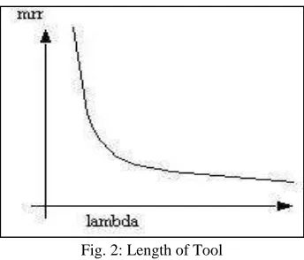
Fig. 2: Length of Tool
The mass length of the tool is very important. Too great a mass absorbs much of the ultrasonic energy, reducing the efficiency of machining. Long tool causes overstressing of the tool. Most of the USM tools are less than 25 mm long. In practice the slenderness ratio of the tool should not exceed 20. The under sizing of the tool depends coupon the grain size of the abrasive. It is sufficient if the tool size is equal to the hole size minus twice the size of the abrasives.
Boron carbide is by far the fastest cutting abrasive and it is quite commonly used. Aluminium oxide and silicon carbide are also employed. Boron carbide is very costly and its about 29 times higher than that of aluminium oxide or silicon carbide. The abrasive is carried in slurry of water with 30-60% by volume of the abrasives. When using large-area tools, the concentration is held low to avoid circulation difficulties. The most important characteristic of the abrasive that highly influences the material removal rate and surface finish of the machining is the grit size or grain size of the abrasive. It has been experimentally determined that a maximum rate of machining is achieved when the grain size becomes comparable to the tool amplitude. Grit sizes of 200-400 are used for roughing operations and a grit size of 800-1000 for finishing.
As the tool vibrates with a specific frequency, abrasive slurry (usually a mixture of abrasive grains and water of definite proportion) is made to flow through the tool work interface. The impact force arising out of vibration of the tool end and the flow of slurry through the work tool interface actually causes thousands of microscopic abrasive grains to remove the work material by abrasion. Material removal from the hard and brittle materials will be the form of sinking, engraving or any other precision shape.
II. MACHINING UNIT
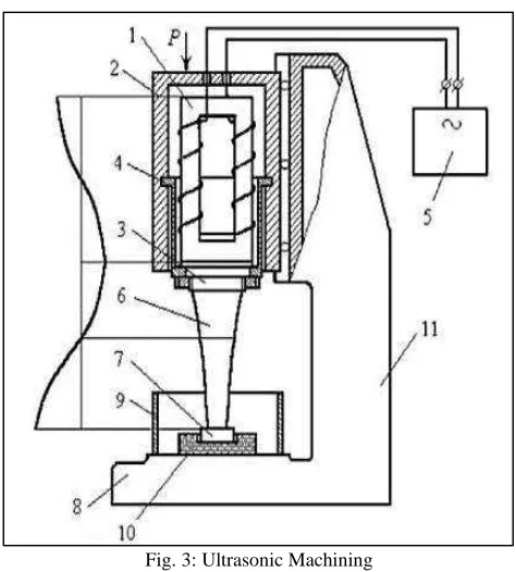
Fig. 3: Ultrasonic Machining
The ultrasonic vibration machining method is an efficient cutting technique for difficult-to-machine materials. It is found that the USM mechanism is influenced by these important parameters.
Amplitude of tool oscillation (a0) Frequency of tool oscillation (f) Tool material
Type of abrasive
Grain size or grit size of the abrasives Feed force - F
Contact area of the tool – A
Volume concentration of abrasive in water slurry – C
Ratio of workpiece hardness to tool hardness; λ=σw/σt λ=tool size, σ=hardness
III. METHODOLOGY
The objective of the present work is to find out main effect of cutting speed, feed rate, drill diameters, work piece material, drill material and interaction effect between drill material and cutting speed on MRR, Surface roughness, Hole diameter error, and burr height. The determination of factors which needs to be investigated depends on the responses of interest. The factors that affect the responses were identified using several methods such as brainstorming, cause and effect analysis and flowcharting. The lists of factors studied with their levels are given in the Table 3.1 the minimum DOF required in the experiment are the sum of all the degrees of freedom of factors and their interaction. In the present experiment setup, there are 4 three level factors and one is 2-level factor i.e tool
Table - 3.1 Input Parameters
Experiment No Tool material Frequency (KHz) Amplitude (micro-meter) Conc. (%)
1 Ti 19 15 30
2 Ti 19 30 35
3 Ti 19 50 40
4 Ti 22 15 30
5 Ti 22 30 35
6 Ti 22 50 40
7 Ti 25 15 30
8 Ti 25 30 35
9 Ti 25 50 40
13 Ca 22 15 30
14 Ca 22 30 35
15 Ca 22 50 40
16 Ca 25 15 30
17 Ca 25 30 35
18 Ca 25 50 40
material The number of DOF for factors A,B, C are two and for factor D is one. The total DOF for the experiment explained in Table 3.2. As the DOF required for the experiment is nine the orthogonal array (OA) to be used should have more than nine dof. The most suitable orthogonal array which can be used for this experiment is L18, which has 17 DOF assigned to its various columns. The additional four DOF used to measure the random error. Taguchi orthogonal arrays are experimental designs that usually require only a fraction of the full factorial combinations. The columns of arrays are balanced and orthogonal. This means that in each pair of columns, all factor combinations occur same number of times. Orthogonal designs allow estimating the effect of each factor on the response independently of all other factors. Once the degrees of freedom are known, the next step is to select the orthogonal array (OA). The number of treatment conditions is equal to the number of rows in the orthogonal array
Table - 3.2
Factors and their levels of interest
Factors Factors designation Level 1 Level 2 Level 3
Tool material A titanium carbide
Frequency B 19 22 25
Amplitude C 15 30 50
Conc. D 30 35 40
and it must be equal to or greater than the total degrees of freedom and experimental design of L18 is shown in Table 3.1 Response factor has to be calculated and the response characteristics given in the Table 3.3
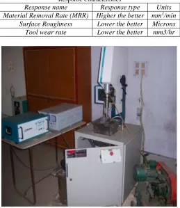
Table - 3.3 Response Characteristics
Response name Response type Units
Material Removal Rate (MRR) Higher the better mm3/min Surface Roughness Lower the better Microns
Tool wear rate Lower the better mm3/hr
Fig. 4: Experimental Setup
IV. RESULTS AND ANALYSIS
Results for MRR
The results for MRR for each of the 18 treatment conditions with repetition and MRR of each sample is calculated from weight difference of work piece before and after the performance trial. The results for MRR were analyzed using ANOVA for identifying the significant factors affecting the performance measures. The Analysis of Variance (ANOVA) for the mean MRR at 95% confidence interval is given in Table 4.1. The variance data for each factor and their interactions were P value to find significance of each. From Table 4.1 tool material (A), amplitude (C) and concentration (D) have the P value less the 0.05 that means these factors are significant. Interaction between tool material and frequency has the P value more than the 0.05 that means this factor is insignificant. Frequency has value of P more than 0.05 that means it is insignificant.
Table - 4.1 ANNOVA for MRR
Source SS v V F P SS' % contribution Status
Tool material (A) 4.292 1 4.292 4.25 0.043 3.002 2.90 Significant
frequency (B) 4.716 2 2.358 2.34 0.159 Insignificant
amplitude (C) 72.165 2 36.083 35.75 0.000 69.585 67.27 Significant
conc (D) 11.487 2 5.744 5.69 0.029 8.907 8.610 Significant
Tool material × frequency (E) 2.713 2 1.357 1.34 0.314 Insignificant
Residual error 8.074 8 1.009
Total 103.448 17
E-pooled 15.503 12 1.29
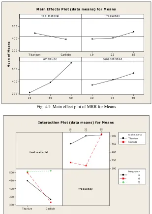
Fig.1 and Fig.2 shows the main effect plot of MRR for Means and interaction plot for MRR. Fig.3 shows the main effect plot for MRR of S/N ratio
Fig. 4.1: Main effect plot of MRR for Means
M e a n o f M e a n s
Carb id e T it an iu m
6 0 0
4 0 0
2 0 0
2 5 2 2 1 9 5 0 3 0 1 5 6 0 0
4 0 0
2 0 0
4 0 3 5
3 0
t o o l m at e rial fre q u e n c y
am p lit u d e c o n c e n t rat io n
M ain Effe cts P lot (data means) for M e ans
t o o l m a t e ria l
fre q u e nc y
25 22 19 500 450 400 350 300
C a rbide Tita nium 500 450 400 350 300
to o l material T itan iu m C arb id e
freq u en c y
25 19 22
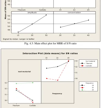
Fig. 4.3: Main effect plot for MRR of S/N ratio
Fig. 4.4: Interaction plot for MRR of S/N ratio
Optimal Design
The same level of all the significant factors provide a higher mean value and reduced variability so nothing has to be compromised. The level of factors which improves average and uniformity may conflict, so a compromise may have to be reached. Also a compromise has to occur when multiple responses are considered and the same factor level may cause one response to improve and other to reduce. In this experimental analysis, the main effect plot in Figure 4.1 is used to estimate the mean MRR with optimal design conditions. In Table 4.2 it is concluded that highest MRR was achieve at amplitude of 50 micro-meters with 40% of slurry concentration and with titanium tool. In S/N ratio highest MRR was found at 25 KHz frequency, 50 micro-meter of amplitude and 40% of slurry concentration. MRR is a “Higher the better” type response. In this experiment analysis, different experimental trials have been chosen to obtain satisfactory results. After conducting the experiments, the optimum treatment condition within the experiments determined based on prescribed combination of factor levels is determined to one of those in the experiment.
Table - 4.2
Significant factors and interactions for MRR
Factor Affecting mean Affecting variation
contribution Best level contribution Best level Tool material (A) significant level 1(Ti) insignificant
Frequency (B) insignificant significant Level 3(25)
amplitude (C) significant Level 3(50) significant Level 3(50) Conc. (D) significant Level 3(40) significant Level 3(40) Tool material*frequency (E) insignificant insignificant
M e a n o f S N r a ti o s
Carb id e T it an iu m
5 6 5 4 5 2 5 0 4 8 2 5 2 2 1 9 5 0 3 0 1 5 5 6 5 4 5 2 5 0 4 8 4 0 3 5 3 0
t o o l m at e rial fre q u e n c y
am p lit u d e c o n c e n t rat io n
M a in Effe cts P lot (da ta me a ns ) for S N r a tios
S igna l-to-noise : La rge r is be tte r
t o o l m a t e ria l
fre q u e n c y
25 22 19 53 52 51 50
C a rbide Tita nium
53
52
51
50
to o l m ater ial T itan iu m C ar b id e
fr eq u en c y
25 19 22
Inte r a ction P lot (da ta me a ns ) for S N r a tios
V. RESULTSANDCONCLUSION
The effect of parameters i.e. tool material, frequency, amplitude and concentration were evaluated using ANOVA design analysis and Regression analysis. The purpose of the ANOVA was to identify the important parameters in prediction of MRR. Some results consolidated from ANOVA and plots are given below
The effect of parameters i.e. tool material, frequency, amplitude and conc. were evaluated using ANOVA and factorial design analysis. A confidence interval of 95% has been used for the analysis. Two repetitions for each 18 trails were completed to measure the Signal to Noise ratio (S/N Ratio).
ANOVA table shows that tool material with F value 4.25, amplitude with F value 36.08 and concentration 5.74 are the factors that significantly affect the MRR, with % contribution of 2.9%, 67.27 % and 8.61% to MRR
The other factor frequency was found to be insignificant. For S/N ratio frequency, amplitude and concentration are significant to reduce the variation of MRR.
So the confidence interval around the MRR is given by 8.52 ± 1.43 mm3/min.
The present study was carried out to study the effect of input parameters on the MRR and surface roughness and tool wear rate. The following conclusions have been drawn from the study:
MRR is mainly affected by type of tool material, amplitude and conc..
REFERENCES
[1] G. Eason, B. Noble, and I. N. Sneddon, “On certain integrals of Lipschitz-Hankel type involving products of Bessel functions,” Phil. Trans. Roy. Soc. London, vol. A247, pp. 529–551, April 1955. (references)
[2] J. Clerk Maxwell, A Treatise on Electricity and Magnetism, 3rd ed., vol. 2. Oxford: Clarendon, 1892, pp.68–73.
[3] I. S. Jacobs and C. P. Bean, “Fine particles, thin films and exchange anisotropy,” in Magnetism, vol. III, G. T. Rado and H. Suhl, Eds. New York: Academic, 1963, pp. 271–350.
[4] K. Elissa, “Title of paper if known,” unpublished.
[5] R. Nicole, “Title of paper with only first word capitalized,” J. Name Stand. Abbrev., in press.
[6] Y. Yorozu, M. Hirano, K. Oka, and Y. Tagawa, “Electron spectroscopy studies on magneto-optical media and plastic substrate interface,” IEEE Transl. J. Magn. Japan, vol. 2, pp. 740–741, August 1987 [Digests 9th Annual Conf. Magnetics Japan, p. 301, 1982].