Image Inpainting Based on Sparse Representation with
Histogram Dictionary
Qiaoqiao Li
1*, Guoyue Chen
2, Xingguo Zhang
2, Kazuki Saruta
2, Yuki Terata
21The Graduate School of Systems Science and Technology, Akita Prefectural University, Akita, Japan. 2Dept. of Electronics and Information Systems, Akita Prefectural University, Akita, Japan.
* Corresponding author. Email: [email protected]
Manuscript submitted May 10, 2018; accepted July 8, 2018. doi: 10.17706/jcp.13.10 1145-1155.
Abstract: This paper proposes a novel image inpainting algorithm based on sparse representation with histogram dictionary. In the propose method, it is a patch-based inpainting method, a patch as the basic unit of inpainting algorithm. Instead of using all the known image patches to form a dictionary, we propose to construct a histogram dictionary by using the histogram. If the histogram between an image patch which cuts from the source region of the input image and the target patch are similar, the image patch as the similar patch is selected to generate a similar dictionary for inpainting algorithm. Two kinds of similarity methods are proposed, so two kinds of histogram dictionaries are corresponding. These histogram dictionaries can ensure a large related to the target patch. Experimental results show that the proposed inpainting method using the histogram dictionary can efficiently inpainting of missing areas.
Key words: Image inpainting, sparse representation, histogram dictionary, similarity.
1.
Introduction
The filling-in of missing or corrupted region in an image, which is cased image inpainting and is an inverse ill-posed problem, is an import topic in the field of computer vision and image processing [1]-[7]. Image inpainting, has been extensively investigated in the applications of digital effect (e.g., object removal), image coding and transmission (e.g., recovery of the missing block), image restoration (e.g., scratch or text removal in photograph), etc. [1]-[3].
region, some blur will be introduced in the texture or large missing region.
In the exemplar-based inpainting method, this kind of methods are inspired by the idea of texture synthesis technique [8]. These algorithms see the image patch as a unit, and the basic idea of these algorithms is finding the best match patch to inpaint the missing areas. As we all known, a natural image is composed of structural information suitable and texture information. According this fact, Bertalmio et.al [9] proposed a method which decomposes the image into structure layer and texture layer. Then they employed the method of diffusion [1] to inpaint the structure layer, and used the technique [8] to process the texture layer. After that, the two reconstructed images are added back together to obtain the inapitning result. Criminisi et. al [10], [11] proposed an exemplar-based inpainting algorithm, in order to preserve the structure information they defined image patch priority. Le Meur et. al [12] improved the filling order based on structure tensor, and applied the new filling order for their exemplar-based inpainting. Xu et.al [13] proposed a method by patch propagation by using a modified filling-in order and inpainted the missing area using the sparse linear combination of candidate patches. Deng et. al [14] proposed an exemplar-based image inpainting method by using a new priority definition which separates the Criminisi’s priority definition into two phases. However, the traditional exemplar-based methods which find a best match patch and copy pixel values to restore the corrupted patch directly. It can cause the unwanted information to the inpainting patch. Moreover, searching the whole image to find a best match patch is time consuming.
Recently, sparse representation has introduced into image inpainting [2], [5], [15]-[20]. The main point of this method is to represent the image patches by using a sparse linear combination of atoms from a dictionary. Thus, the dictionary is very important for inpainting results. Amano et. al [18] utilized the learning samples which were clipped from the local region (where has no defect region) as eigenvector series in their interpolation method and obtained the good image interpolation results. Shen et. al [19] directly used all the patches in the source region to construct a dictionary and obtained a good inpainting results. However, the dictionary contains all the patches which are in the source region, it will have some of unrelated atoms with an image patch to be restored. Moreover, the unrelated atoms will introduce the interference into inpainting results. Aharon et. al [20] proposed a K-SVD algorithm for designing dictionaries for sparse presentation. Mairal et. al [16] introduced a sparse representation for color image restoration by using the K-SVD algorithm. However, this method is suitable for denoising, but is not suitable for inpainting.
2.
Preliminaries
Recently, signal sparse representation has attracted many researches’ attention. And a patch is always set to a basic unit in signal sparse representation [5], [20], [21].
Given a dictionaryDwhose columns are prototype signal-atoms atoms D[ ,d1 ,dk], a patchycan be represented as a sparse linear combination of these atoms, that is,
y Dα (1) whereαare the sparse representation coefficients of the patch.
Considering the inpainting problem, some pixels of the image patch are damaged. Therefore, we can divide the patchyinto the known pixels and missing pixels, respectively. DenoteMas a matrix to extract
the known pixels iny
*
y My (2)
In the problem of image inpainting, we want to use the known pixels *
y to estimate the patchy. First,
infer the sparse coefficientsαby minimizing an optimization problem
0 . .
min‖ ‖ s t y*MDα
α α (3)
where ‖‖0means l0 norm which counts the nonzero elements inα. Because the problem of l0 norm is usually an NP-hard problem [22], thus it is often solved by greedy algorithms such as matching pursuit (MP) [23] and the orthogonal matching pursuit (OMP) [24] algorithms.
Second, after obtaining the estimation of coefficientsαˆ, the image patchycan be reconstructed from its sparse coefficientsαˆby using
ˆ , ˆ, if i if i * * i * y y MDα y i
y (4)
where Mis a matrix which is determined the location of missing pixels.
3.
Histogram Dictionary
In this section, we will introduce how to flexibly construct a histogram dictionary for a target patchΨpin the given imageI.
First, select a target patchΨpusing the filling order which is described by Criminisi et. al [10], [11] and compute the histogram of it. Let the histogram have N bins. Therefore, the histogram of color image has N values. For three channels R, G, B of target patchΨp, the histogram of each channel can be represented by
R [ R1, , R ]
T N
h h
p p p
Ψ Ψ Ψ
h
G [ G1, , G ]
T N
h h
p p p
Ψ Ψ Ψ
h (5)
B [ B1, , B ]
T N
h h
p p p
Ψ Ψ Ψ
h
Second, cut the whole known patches fi (i 1, , l) from the imageIand compute the histogram of
them (withLdenotes the number of known patches). fRi, fGiand fBi denote three channels (RGB) of the
patch, respectively. The histogram of each channel can be represented by
R 1 R
[ , , ] i iN T f f h h Ri f h
[ Gi1, , Gi ] T
f f N
h h
Gi
f
h (6)
B 1 B
[ , , ] i iN T f f h h Bi f h
R R 1 R R
1
|| || (| |)
i p j fij
j
h h
p
Ψ f h h
Ri
v
1 G G 1
|| || (| |)
p ij
N
j f
j
h h
p Gi
Ψ G f h h
Gi
v (7)
B
B 1 B
1
|| || (| |)
p ij
N
j f
j
h h
p Bi
Ψ f h h
Bi
v
The aim is to find out the similar patches from the whole candidate patches, so how to select the similar patch is a problem.
In order to solve this problem, two similarity method by using histogram are proposed.
3.1.
Similarity Based on Sum
The similarity based on sum vSiis defined as
vSi=vRi+vGi+vBi (8) Considering the number of the known patches isl, the similarity based on sum is written by
vS
vS1, ,vSl
T (9)a. Target patch 1 and its chosen patches b. Target patch 2 and its chosen patches
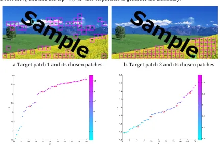
c. Chosen patches of (a) are shown in scatter plots d. Chosen patches of (b) are shown in scatter plots Fig. 1. The chosen patches by using sum histogram.
In order to see clearly which patches are chosen for generating the dictionary, we mark out the top 50
t most similar sample patches which are used to construct a histogram dictionary. That is to say, the sample patch 1 is the first similar to the target patch and so on. The result is shown in Fig. 1. Fig. 1 (a) and Fig. 1 (b) are shown one target patch (blue-green) and its top 50 chosen patches (mulberry). Fig. 1 (c) and Fig. 1 (d) are shown the chosen patches of the two samples by using the similarity based on sum in scatter corresponding bins of the histogram. In R, G, Bthree channels, the difference can be defined by comparing their histogram as follows:
plots.
3.2.
Similarity Based on Max
Considering the three channels of the color image, we see the similarity of patches as a 3-D vector and find the maximum value of it. The similarity based on max vMi is defined as
( , , )
max
Mi Ri Gi Bi
v v v v (10)
Considering the number of the known patches is L, the similarity based on max is written by
vM
vM1, ,vMl
T (11) Then, sort vM and find the top t (t < l) known patches to generate the dictionary.For 3-D case, in Fig. 2 (a) -(b) are shown the top t50 sample patches which are constructed a histogram dictionary for the two target patches by comparing similarity based on max. In Fig. 2 (c) -(d) are shown the chosen patches of the two samples by using similarity based on max in scatter plots.
a. Target patch 1 and its chosen patches b. Target patch 1 and its chosen patches
c. Chosen patches of (a) are shown in scatter plots d. Chosen patches of (b) are shown in scatter plots
Fig. 2. The chosen patches by using max histogram.
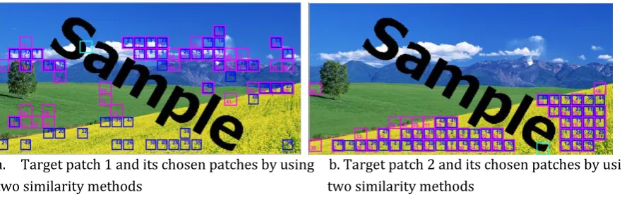
a. Target patch 1 and its chosen patches by using b. Target patch 2 and its chosen patches by using two similarity methods two similarity methods
Using the two different methods to comparing the similarity, the histogram dictionary will be different. In order to view the patches are chosen to form histogram dictionary with comparing similarity method easily, Fig. 3 is shown the chosen top 50 patches with the two similarity methods in the same picture. The mulberry block is shown the results of based on max method and the blue block are shown the based on sum method, respectively. From Fig. 3 (a), the chosen top 50 sample patches by using similarity based on max contain more relevant patches than that by using similarity based on sum. From Fig. 3 (b), the chosen top 50 sample patches by using similarity based on max are generally as relevant as the chosen patches by using similarity based on sum.
4.
Overview of the Proposed Algorithm
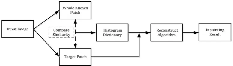
Furthermore, a new image inpainting method is proposed based on this histogram dictionary. As discussed above, the schematic diagram of the proposed inpainting algorithm is shown in Fig. 4.
The detailed procedures of the proposed method are as follows:
First, input the inpainting image which is denoted byI. And the imageI contains the source regionS (undamaged region) and the target regionT (damaged region). That is to say
I S T (12) Second, provide a window size of n × n and cut the patches from the source regionS, and then a group of known patches { } 1
l i i
f can be obtained.
*
p p
Ψ MΨ (13) Fourth, compare the similarity between the target patch and the all known patches by using the methods which are described in the section III. And then select the m similar patches to create a histogram dictionary for the target patch. The size of histogram dictionary is 2
n m (m < l) which is denoted byDh. Because there are two similar methods for proposed inpainting method, the histogram dictionariesDhare
also two kinds. The histogram dictionary using similarity based on sum is denoted byDhSand histogram
dictionary using similarity based on sum is denoted byDhM, respectively.
Fig. 4. Schematic diagram for the proposed inpainting algorithm.
Finally, estimate the sparse coefficientsαˆ by using the non-negative orthogonal matching pursuit algorithm (NNOMP) [25] which is an improved method of OMP [24]. Reconstructing the target patchΨpfrom the sparse coefficientsαˆis expressed as:
ˆ ,
ˆ ,
if i
if i
i
i p
p
h Ψ Ψ
MD α
S
T (14)
4.1.
Image Inapainting Algorithm
In the light of introduction above, the proposed method based on sparse representation by using histogram dictionary is described in detail in Algorithm 1. Here, we adopt the histogram dictionaryDhMby
using the similarity based on max to explain. For the histogram dictionaryDhSjust replacing the similarity
based on sum vMto the similarity based on sumvS, the process is same.
Algorithm 1 The proposed method based on sparse representation by using histogram dictionary 1: Input: the observed imageI
2: initialization: block=n n ,KP,l0
3: Repeat:
4: clipped the patchfl +1from the image I in a window(n n )
5: if fl +1 is in the source region Sof the image I
6: fl +1 is as a candidate patch
7: compute the histogram of the patch by equation (6) 8: l l 1
9: updateKPl +1[KPl fl +1]
10: end if
11: until
12: Iteration: the window scans the bottom right corner 13: while Ihas defective pixels do
14: initialization: vM [ ]
15: use the filling order to find the target patchΨp 16: compute the histogram of it by equation (5) 17: for i1 :l
18: compute the difference between the target patch and the candidate patches by equation (7) 19: use vMi max(vRi,vGi,vBi)
20: update vM [vM vMi] 21: end for
22: sort the maximum value by 23: indexsort(vM)
24: obtain the histogram dictionary by 25: DhKP(:,index(1: ))l
26: estimate the sparse coefficient by 27: αˆFNNOMP(ψp,Dh)
28: reconstruct theψp by using equation (14) 29: end while
30: Output: inpainting imageIˆ
5.
Experiment Results
the proposed method with Criminisi’s [10], [11] inpainting algorithm. The proposed method is also employs the inpainting filling order which is described in [10], [11]. And the proposed method is implemented by using Algorithm 1 based on the schematic diagram in Fig. 5. The number of L is set as 400, that is to say we choose the top 400 patches as the similar dictionary. For fairness, the window size of all methods are set 9 9 .
The performance of the proposed method is compared with different image inpainting methods in quantitative evaluations. We use the peak signal-to-noise ratio (PSNR) as the metrics to evaluate the imapinting results. Furthermore, in order to see clearly, PSNR values in three channels (R, G, B) are also presented. The larger the value of the PSNR, the better the inpainting result.
a b c
Fig. 5. Obtained results of three natural images. The first row shows three original images. The second row shows the degraded images. The third to fifth row show the result of Criminisi, the proposed method based
on histogram dictionaryDhSand the proposed method based on histogram dictionaryDhM.
Considering the two similar methods, the proposed method inpaint the missing region by using the histogram dictionaryDhSandDhM. Fig. 6 presents three testing images for this experiment. The first row is
corrupted images, results of Criminisi’s inpainting algorithm [10], [11], the proposed method by using the histogramDhSand the proposed method by using the histogramDhM. The peak signal-to-noise ratio
(PSNR) between the result and the original image is summarized in Table 1. It can be seen in Fig. 6, the Criminisi’s algorithm cause obvious miscopies in the third row. For instance, the snow mountain in (c) of the third row appears unwanted structure of the Criminis’s result. This is because the Criminisi’s method only chooses a best match patch to inpaint missing region, some unwanted artifacts appear the results. In the fourth row, the result of the proposed method by using the histogram dictionaryDhSis shown. The edge
of the mountain is not inpainted very well in (a) of the fourth row. And in (c) of the fourth row, extra color produces in the result. For the proposed method by using the histogram dictionaryDhM, the similar patches
are chosen by similarity based on max in the framework of sparse representation, so it can overcome the influences which caused by Criminisi’s inpainting method. Furthermore, the histogram dictionaryDhMis
generated by comparing the difference in 3-D vector, it is more suitable for the color image than the histogram dictionaryDhSfor the proposed method. And the fact confirms the quantitative metrics as shown
in Table 1. The objective quantitative evaluation is consistent with the subjective visual effect of the inpainting result images.
Table 1. Objective Performance
Image RGB Criminisi Sum Max
Image 1
R 38.8751 40.8970 41.3303
G B RGB
38.4905 39.0629 38.8095
39.7892 39.9818 40.2227
40.7463 40.9369
41.0045
R 24.3601 25.5961 25.6186
G 26.0846 27.3549 27.3753
Image 2 B 32.5088 32.1619 33.7642
RGB 27.6512 28.3710 28.9194
R 24.4232 24.4091 26.7018
G 24.8705 30.2230 30.2815
Image 3 B 29.2284 32.2277 32.1201
RGB 27.1740 28.9533 29.7011
6.
Conclusion
In this paper, we have proposed a new inpainting method based on sparse representation. In this paper, two measure similarity methods, i.e. based on sum and similarity based on max, are proposed for comparing the similarity between the target patch and the all candidate patches. And then the similar patches are chosen to form a histogram dictionary. In this way, the interference of the non-related patches to the sparse construction to be avoided. The proposed inpainting method using the histogram dictionary shows good performance both in the PSNR sense and visually when compared with the Criminisi’s method.
Acknowledgment
This work was supported by the China Scholarship Council (CSC 201708050084).
References
[2] Fadili, M. J., Starck, J. L., & Murtagh, F. (2007). Inpainting and zooming using sparse representations. The Computer Journal, 52(1), 64-79.
[3] Guillemot, C., & Meur, O. L. (2014). Image inpainting: Overview and recent advances. IEEE Signal Processing Magazine, 31(1), 127-144.
[4] Zhang, J., Zhao, D., & Gao, W. (2014). Group-based sparse representation for image restoration. IEEE Transactions on Image Processing, 23(8), 3336-3351.
[5] Xu, K., Wang, N., & Gao, X. (2016). Image inpainting based on sparse representation with dictionary pre-clustering. Proceedings of Chinese Conference on Pattern Recognition. Springer (pp. 245-258). [6] Bertalmio, M., Bertozzi, A. L., & Sapiro, G. (2001) Navier-stokes, fluid dynamics, and image and video
inpainting. Proceedings of the 2001 IEEE Computer Society Conference on Computer Vision and Pattern Recognition.
[7] Chan, T., & Shen, J. (2001). Local inpainting models and tv inpainting. SIAM J. Appl. Math, 62(3), 1019-1043.
[8] Efros, A. A., & Leung, T. K. (1999). Texture synthesis by non-parametric sampling in computer vision. Proceedings of the Seventh IEEE International Conference (pp. 1033–1038).
[9] Bertalmio, M., Vese, Sapiro, L. G., & Osher, S. (2003). Simultaneous structure and texture image inpainting. IEEE Transactions on Image Processing, 12(8), 882-889.
[10] Criminisi, A., Perez, P., & Toyama, K. (2004). Region filling and object removal by exemplar-based image inpainting. IEEE Transactions on Image Processing, 13(9), 1200-1212.
[11] Criminisi, A., Perez, P., & Toyama, K. (2003). Object removal by exemplar-based inpainting. Proceedings of IEEE Computer Society Conference on Computer Vision and Pattern Recognition (pp. II–II) .
[12] Meur, O. Le., Gautier, J., & Guillemot, C. (2011). Examplar-based inpainting based on local geometry. Proceedings of the 18th IEEE International Conference on Image Processing (ICIP) (pp. 3401-3404). [13] Xu, Z., & Sun, J. (2010). Image inpainting by patch propagation using patch sparsity. IEEE Transactions
on Image Processing, A Publication of the IEEE Signal Processing Society, 19(5), 1153-1165.
[14] Deng, L. J., Huang, T. Z., & Zhao, X. L. (2005). Exemplar-based image inpainting using a modified priority definition. Plos One, 10(10).
[15] Elad, M., Starck, J. L., Querre, P., & Donoho, D. L. (2005). Simultaneous cartoon and texture image inpainting using morphological component analysis (mca). Applied and Computational Harmonic Analysis, 19(3), 340-358.
[16] Mairal, J., Elad, M., & Sapiro, G. (2008). Sparse representation for color image restoration. IEEE Transactions on Image Processing, 17(1), 53-69.
[17] Ogawa, T., & Haseyama, M. (2013). Image inpainting based on sparse representations with a perceptual metric. EURASIP Journal on Advances in Signal Processing, 2013(1), 179.
[18] Amano, T., & Sato, Y. (2007). Image interpolation using bplp method on the eigenspace. Systems and Computers in Japan, 38(1), 87-96.
[19] Shen, B., Hu, W., Zhang, Y., & Zhang, Y.-J. (2009). Image inpainting via sparse representation. Proceedings of IEEE International Conference on Acoustics, Speech and Signal Processing (pp. 697-700).
[20] Aharon, M., Elad, M., & Bruckstein, A. (2006). rmk-svd: An algorithm for designing overcomplete dictionaries for sparse representation. IEEE Transactions on Signal Processing, 54(11), 4311-4322. [21] Elad, M., & Aharon, M. (2006). Image denoising via sparse and redundant representations over
learned dictionaries. IEEE Transactions on Image processing, 15(12), 3736-3745.
Approximation, 13(1), 57-98.
[23] Mallat, S., & Zhang, Z. (1993).Matching pursuits with time-frequency dictionaries. IEEE Transactions on Signal Processing, 41(12), 3397-3415.
[24] Tropp, J. A., & Gilbert, A. C. (2007). Signal recovery from random measurements via orthogonal matching pursuit. IEEE Transactions on Information Theory, 53(12), 4655-4666.
[25] Yaghoobi, M., Wu, D., & Davies, M. E. (2015). Fast non-negative orthogonal matching pursuit. IEEE Signal Processing Letters, 22(9), 1229-1233.
Qiaoqiao Li received the B. Eng. degree from Zhengzhou University, Zhengzhou, China, in 2012, and the M. Eng. degree from Lanzhou University, Lanzhou, China, 2016. She is currently pursuing Dr. Eng. degree at Akita Prefectural University, Akita, Japan. Her research interests include signal processing and image Processing.
Guoyue Chen received his B.Sc degree from East China Normal University, China, in 1983, where he worked as a research associate at the Department of Computer Science until 1989. He received his M.S and Ph.D degrees from Tohoku University, Japan in 1993 and 1996, respectively. He is currently a professor in Akita Prefecture University, Japan. His interests include digital signal processing and its applications to active noise control, and image processing.
Xingguo Zhang received the B.E. degree in computer science from the Dalian Polytechnic University of China in 2009, and the M.E and Ph.D degrees from the Akita Prefectural University of Japan in 2012 and 2015. Currently, he is a teaching assistant in Akita Prefectural University, Japan. His research interests include computer vision, pattern recognition, and machine learning.
Kazuki Saruta received his BE and ME degrees from Akita University, Japan, in 1991 and 1993, and his Ph.D degree from Tohoku University, Japan, in 1996. Then, he was a lecturer in the Faculty of Humanities of Yamagata University. In 1999, he was invited as an associate professor in the Department of Electronics and Information Systems of Akita Prefectural University, Japan. He has been engaged in research on pattern recognition and image processing.