Hall Current Effects on Peristaltic Transport of A Conducting Bingham Fluid With Permeable Walls By Adomian Decomposition Method

IJSRR, 7(4) Oct. – Dec., 2018 Page 179

Research article Available online www.ijsrr.org

ISSN: 2279–0543

International Journal of Scientific Research and Reviews

Hall Current Effects on Peristaltic Transport of A Conducting

Bingham Fluid With Permeable Walls By Adomian Decomposition

Method

Laxmi Devindrappa

and Naduvinamani N. B.

Department of Studies and Research in Mathematics, Gulbarga University, Kalaburagi-585106, Karnataka, India

E-mail: [email protected] , [email protected]

ABSTRACT

The influence of Hall current effect on peristaltic transport of a conducting Bingham fluid with permeable walls by Adomian decomposition method is examined. The non linear partial differential equations that govern that model were simplified under assumptions of long wavelength and low Reynolds number. This model is suitable for the blood flow in the sense that erythrocytes region and the plasma regions can be described as plug flow and non-plug flow regions. The velocity field for the model of interest is solved by Adomian decomposition method. The pressure gradient, pressure rise, stream functions and frictional force are discussed with the help of graphs drawn for different parameters like Darcy number, Hall parameter, Hartmann number and Slip parameter.

KEYWORDS:

NOMENCLATURE

b : Amplitude

c : Wave speed

F : Frictional force

m : Hall parameter

M : Hartmann number

Q : Time averaged flow rate

e

R : Reynolds number

 : Wavelength

i j

 : Stresses

0

 : Yield stress.

 : Slip parameter

p

 : Pressure rise

a

D : Darcy number.

*Corresponding author

Laxmi Devindrappa

Department of Studies and Research in Mathematics, Gulbarga University, Kalaburagi-585106, Karnataka, India

IJSRR, 7(4) Oct. – Dec., 2018 Page 180

INTRODUCTION

Peristalsis is a series of wave-like muscle contractions that moves food to different

processing stations in the digestive tract. The process of peristalsis begins in the esophagus when a

bolus of food is swallowed. The strong wave-like motions of the smooth muscle in the esophagus

carry the food to the stomach, where it is churned into a liquid mixture called chyme. Next,

peristalsis continues in the small intestine where it mixes and shifts the chyme back and forth,

allowing nutrients to be absorbed into the bloodstream through the small intestine walls. Peristalsis

concludes in the large intestine where water from the undigested food material is absorbed into the

bloodstream. Finally, the remaining waste products are excreted from the body. The mechanics of

peristalsis has been examined by a number of investigators. Latham1 was probably the first to investigate the mechanism of peristalsis in relation to mechanical pumping. Fung and Yih2 presented a theoretical analysis of peristaltic transport primarily with inertia-free Newtonian flows driven by

sinusoidal transverse waves of small amplitude. Investigation of peristaltic motion in connection

with functions of different physiological systems such as the ureter, the gastro-intestinal tract, the

small blood vessels and other glandular ducts was first made by Shapiro et al.3.

The fluid mechanical description of the esophageal peristaltic transport with the help of

two-fluid model has been explained by Brasseur4. Bugliarello and Sevilla5 and Cockelet6 have experimentally shown that blood has a peripheral layer of plasma and a core region of suspension of

all the erythrocytes when it flows through small blood vessels. Srivastava and Srivastava7 have investigated the problem of peristaltic transport of blood in a uniform and non-uniform geometries

by considering blood as a two layered fluid model consisting of a central layer of suspension of all

erythrocytes, etc assumed to be a Casson fluid, which is a yield stress fluid and a peripheral layer of

plasma as a Newtonian fluid. Comparani and Mannucci8 have analyzed the flow of a Bingham fluid in contact with a Newtonian fluid in a channel. Electro-Kinetically driven peristaltic transport of

viscoelastic physiological fluids through a finite length capillary analysed by Tripathi et al.9 . Vajravelu et al.10 studied the peristaltic pumping of a Casson fluid in an elastic tube. Rathod and Laxmi11 have studied the effects of heat transfer on the peristaltic MHD flow of a Bingham fluid through a porous medium in a channel.

If a particle is at rest in presence of magnetic field, the field has no effect. Similarly, if the

particle path is in the same direction as that of the magnetic field, there is no effect i.e. the particle

motion will be undeflected. But if the particle path has a component normal to the direction of

IJSRR, 7(4) Oct. – Dec., 2018 Page 181 angle to the direction of motion of a charged particle, the particle is deflected in a circular path. In

addition to this deflection the particle experiences the electric field. The combined force acting on

the particle is said to be Lorentz force. Conductivity normal to the magnetic field is reduced due to

the free spiraling of electrons and ions about the magnetic lines of force before suffering collisions

and a current is induced in direction normal to both the electric and magnetic fields. This

phenomenon is called the Hall Effect. When the magnetic field is very strong the Hall Effect cannot

be neglected. Hayat et al.12 have investigated the peristaltic flow of a Maxwell fluid including the Hall Effect through porous medium. Asghar et al.13 studied the effects of Hall current and heat transfer on flow due to a pull of eccentric rotating disk. The effect of Hall currents on interaction of

pulsatile and peristaltic transport induced flows of a particle fluid suspension that had been examined

by Gad14. Hussain et al.15 studied the Heat and mass transfer analysis in variabl eviscosity peristaltic flow with Hall current and ion slip. Ellahi et al.16 examined theoretically the peristaltic flow of Jeffrey fluid in a non-uniform rectangular duct under the effects of Hall and ion slip. Hall effects on

peristalsis of boron nitride-ethylene glycol nanofluid with temperature dependent thermal

conductivity investigated by Abbasi et al.17.

With the above discussion in mind, the purpose of the present investigation is to analyse the

Hall current effects on peristaltic transport of a conducting Bingham fluid with permeable walls by

Adomian decomposition method under the assumptions of long wavelength and low Reynolds

number. The expressions for the velocity field and pressure gradient are obtained analytically. The

impact of all the physical parameters of interest is taken into consideration with the help of graphs.

MATHEMATICAL

FORMULATION

Consider the peristaltic pumping of a conducting Bingham fluid in a channel with permeable

walls, under long wavelength and low Reynolds number assumptions. A longitudinal train of

progressive sinusoidal waves takes place on the upper and lower walls of the channel. We assume

that a uniform magnetic field strength B0is applied. For simplicity, we restrict our discussion to the

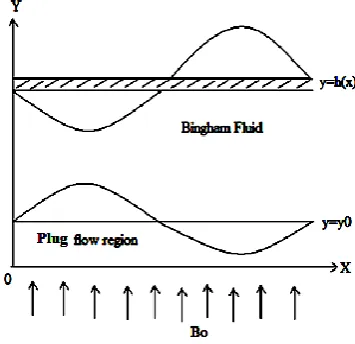
half-width of the channel as shown in the figure.1. The region between y0and yy0is called plug

flow region. In the plug flow region y x 0. In the region between yy0 andyH, _{y x} ₀. The

wall deformation is given by

2

( , ) sin ( )

H X t a b  x ct



   (1)

IJSRR, 7(4) Oct. – Dec., 2018 Page 182 the ends of the channel is a constant, the flow becomes steady in the wave frame ( , )x y moving with

velocity c away from the fixed (laboratory) frame ( , )X Y .The transformation between these two

frames is given by

, , ( , ) ( , ) ( , ) ( , )

x X ct yY u x y U Xct Y and w x y W Xct Y (2)

Where U and W are velocity components in the laboratory frame and u and ware velocity components in the wave frame. In the many physiological situations it is proved experimentally that

the Reynolds number of the flow is very small. So, we assume that the wavelength is infinite. So the

flow is of Poiseuille type at each local cross - section.

Fig. 1. The Physical model

The equations governing the flow in wave frame are given by

0.

u w

x y

 

 

  (3)

 

2 0

2( ).

1

x x y x

u u u p B

u w u c mw

m

t x y x x y

  

_     _       



     

  (4)

2 0

2( ( )).

1

x y y y

w w w p B

u w w m u c

m

t x y y x y

  

_     _       

     

  (5)

Where_m B0

en



 is the hall parameter, e-Electron charge, n-number density of electrons and _{i j} denote the stresses. For the Bingham plastic these are strains through the constitutive model,

.

. y

ij i j



  



 

 

_  _

 

 

for   0and, (6)

. 0 i j i j

IJSRR, 7(4) Oct. – Dec., 2018 Page 183 Where

.

i j



.

, u u_i j i j _{x x}

j i

  

  (8)

1 2 i j i j

    and

2 2

2

. ₁. .

. 2

u w u w

i j i j _{x y y x}

    _ _ _ _ _  _

   

      (9)

0 x y

u y

  

 for   0 ,

0

x y

  for   ₀.

Introducing the non-dimensional quantities

2

0 0

0 0

0 2

, , , , , , , , , ,

, Re , , xx x x, xy x y, yy y y

x y u w pa ct H b a y

x y u w p t h y

a c c c a a a

ca k a a

M aB Da

a c c c

           _ _{    }                     

Into equations (3) to (5), we get (dropping the bars)

0

u w

x y

 

 

  (10)

  2 2 2 Re 1 1 y x x x

u u p M

u w u m w

x y x x y m

 

_    _        

     

  (11)

 

2

3 2

2

Re ( 1)

1

x y y y

w w p M

u w w m u

x y y x y m

   _    _                (12) where . 0 . i j i j               

for   0 (13)

.

0

i j i j

   for   0 (14)

. .

2 x y y x

u u

y x

    

  (15)

. 2 x x u x     , . 2 y y w y   

 (16)

2 2

2 .

2 2

2 u w u w

x y y x

  __ _ _ _{ }_   _

   

     

IJSRR, 7(4) Oct. – Dec., 2018 Page 184

2 2 2

x y x x

    (18)

Under the assumptions of long wavelength and low Reynolds number, the equations (11) to (12)

reduce to

 

2 2

0 1

1

y x

p M

u

x y m



 

    

   (19)

0 p

y   

 (20)

0 x y

u y

  

 for   0 (21)

0

x y

  for   0 (22)

Here 0 is the yield stress.

Here equation (20) indicates that p is independent of yand depends only uponx. Therefore, Eq.

(19), can be rewritten as

 

2 2

2 2 1

1 u dp M

u

y dx m

 _{  }

  (23)

The non-dimensional boundary conditions are

0

u y  



 at y0 (24)

1 Da u

u

y



   

 at yh (25)

Where is slip parameter and _{0 is the yield stress.}

The volume flux qthrough each cross section in the wave frame is given by

0

0

0

y h

p y

q





The instantaneous volume flow rate Q X t( , )in the laboratory frame between the centre line and the

wall is

 

0 0

( , ) 1

H h

Q X t 





IJSRR, 7(4) Oct. – Dec., 2018 Page 185

SOLUTION OF THE PROBLEM

For the solution of Eq. (23), we use Adomian decomposition method, we write Eq. (23) in

operator form   2 2 2 2 1 1 y y

M dp M

L u u

m dx m

  

  (28)

Where L 2₂ y

 

 Since Lis a second-order differential operator,

1

L is a second-fold integration

operator defined by:

   

1

0 0

. .

y y

L 



L , Eq. (28) becomes

 

2 2

1 1

1 2 2 2

1 1

dp M M

u c c y L L u

dx m m

         _  _ _{ }       (30)

In which the function can be determined by utilizing the boundary conditions (24-25). By the

standard Adomian decomposition method, one can write:

0 n n u u   

From eq. (30)

2 2

0 1 2 2

1 2!

dp M y

u c c y

dx m       _    (31)   2 1

1 2 ,

1

n n

M

u L u

m



  _ n0. (32)

from (31) and (32), we obtain

 2  3  4

2 2

1 1 2

1

2! 3! 4!

Ny c Ny dp Ny

u c N

N dx N

 

  _  _

 

(33)

 4  5  6

2 2

2 1 2

1

4! 5! 6!

Ny c Ny dp Ny

u c N

N dx N

    _  _   (34)         

2 2 2 1 2

2 2

1 2

1

2 ! 2 1 ! 2 !

n n n

n

Ny c Ny dp Ny

u c N

n N n dx N n

      _  _    (35)

IJSRR, 7(4) Oct. – Dec., 2018 Page 186

  2   2





1 2

1

cosh c sinh dp cosh 1

u c Ny Ny N Ny

N dx N

 

  _  _ 

  . (36) where

2 2 1 M N m 

 and subject to the boundary conditions (24) and (25) we obtain

2 0,

c 

(37)               2 0 1 2 0 2 1

1 cosh sinh

1

1

cosh sinh sinh cosh 1

Da dp

N y N N y

dx N

c

Da dp

N h N N y N h N N h

N dx N

    _{ }  _ _     _ _       _{ }   _{ }         _{   }  _{   }   (38)

From equations (36, 37 and 38) we obtain





N Da N Sinh N h y

dp Cosh h y

N

dx Cosh h N Da N Sinh N y Cosh h N Da N Sinh N y u N N                     (39)

Taking in equation (39) yy0, we get the velocity in the plug flow region as up





2 0 0 0 2 2 [ ( )] [ ] 1 [ ] [ ] [ ] [ ] y p

N Da N Sinh N h y

dp Cosh h y

N

dx Cosh h N Da N Sinh N y Cosh h N Da N Sinh N y u N N               _  _     

The volume flux qthrough each cross section in the wave frame is given by

 

0

0

1 2 3 4 0 5 6 7

0

y h

p y

dp

q u dy udy h A A A A y A A A

dx

_ _          (40)

Where

 0

1

1 ₃ 0 _{2 2 2}

1

2 [ ] [ ]

1 2

2 [ ]

2 [2 ]

Da N Cosh hN Tan N h y

A Tan

DaN Da N Cosh hN

      _{ }          .

2 2 2

2 2 [2 ]

A   Da N   Cosh hN

 0

3 3

[ [ ] [ ]] [ ]

Log Cosh hN Da N Sinh N h y Sinh hN

A DaN       





N Da N Sinh N h y

N

Cosh hN Da N Sinh hy A N           0 0 5 2 [ ]

Cosh hN h y A

Da N

  



 0

6 4

[ [ ] [ ]]

Log Cosh hN Da N Sinh N h y

A

Da N

   

IJSRR, 7(4) Oct. – Dec., 2018 Page 187

0

0 0

7 2 2

[ ]

1

[ ] [ ]

Cosh Ny

Cosh hN Da N Sinh hy h y A

N N

 



  

 

From Eq. (40) we have

 





 

1 2 3 4 0 5

6 7

q h A A A A y A

dp

dx A A

      



 (41)

The pressure rise and frictional force over one wavelength of the peristaltic are given by

1

0

dp

p dx

dx

 

_

1

0

dp

F h dx

dx

 

 _ _

 



The above integrals numerically evaluated using the MATHEMATICA software.

RESULTS AND DISCUSSION

We have presented a set of Figures 2-16, which describe qualitatively the effects of various

parameters of interest on flow quantities such as pressure gradient, pressure rise per wavelength,

frictional force and stream functions.

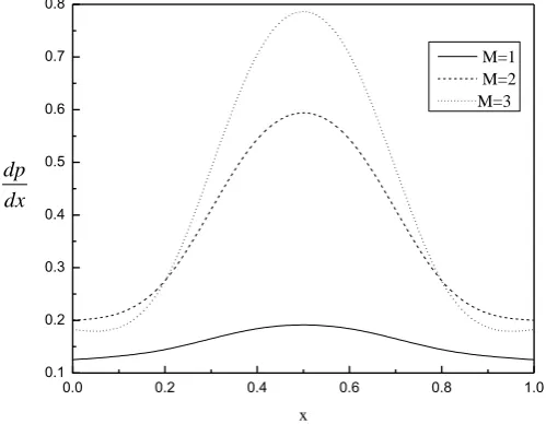
Figures 2–5 show the variations of the axial pressure gradient dp

dx with respect to the axial x

which has oscillatory behavior in the whole range of the x-axis for all other parameters, Figure 2

depicts the impact of Hall parametermon axial pressure gradient. It shows that axial pressure

gradient decreases in the channel. Influence of magnetic field parameterM on pressure gradient

depicted in figure 3. Indeed, the axial pressure gradient increases by increase in M. In Figure 4, It

can be notice that the axial pressure gradient reduces by increase in Da. Figure 5 depicts that dp dxis

increases with the increases of.

The pressure rise per wavelength p against flow rate for different values Hall parameter m,

Darcy numberDa, Hartmann number Mand slip parameter, can be observed from Figs.6-9. It is

observed from the Fig.6, that, in the pumping region the pumping rate decreases by increasing Hall

parameter m, while in the co-pumping region the pumping rate increases by increasing Hall

parameter m, For the free pumping case there are no noticeable difference observed .The variation

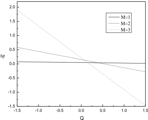
of pressure rise with time averaged flow rate Q for different values of magnetic parameters M is

shown in Fig. 7, it is observed that the larger the magnetic parameter greater the pressure rise against

IJSRR, 7(4) Oct. – Dec., 2018 Page 188 increasing magnetic parameterM. The variation of pressure rise with time averaged flow rate Q for

different values of Da is shown in Fig. 8, for a given pressure rise the flux Q depends on Darcy

number and it decreases with increasing Darcy number Da. For free pumping the flux Q is constant

and it is independent of Da. The variation of pressure rise with time averaged flow rate Q for

different values of  is shown in Fig.9, it is observed that the longer the slip parameter, the greater

the pressure rise against which the pump works. For a given flux Q, the pressure difference p

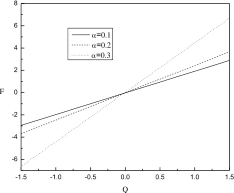
increases with increasing slip parameter. From Figs. 10-13 it can be seen that frictional forces have

opposite behavior as compared to the pressure rise. Formation of circular bolus by internally splitting

of streamlines is known as trapping. The bolus moves forward through peristaltic wave with the

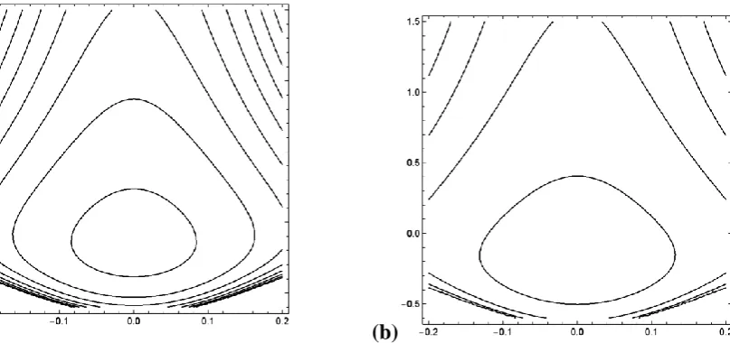
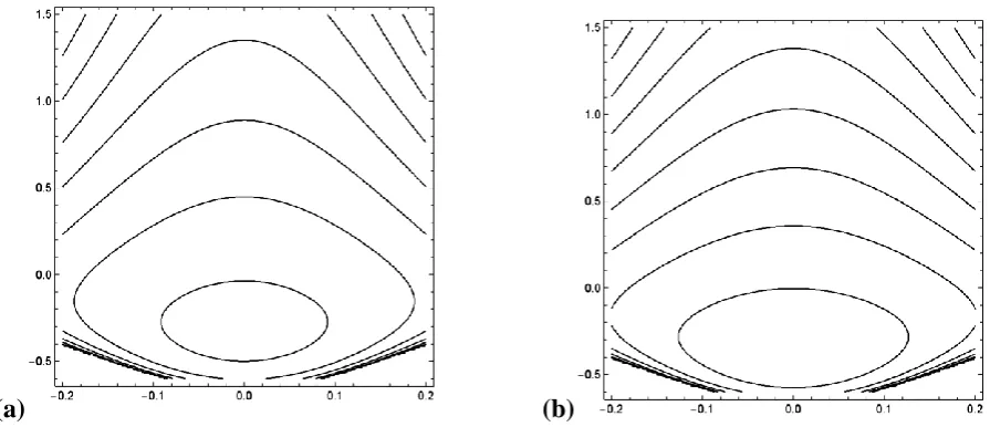
same speed. Figure 14 indicate that for ascending values of Hall parameter m, the size of trapped

bolus becomes larger. Figure 15 indicate indicate that for large value of Hartman number M the size

of trapped bolus increases. Figure 13 depicts that increasing Q led to an increase in trapped bolus

size

CONCLUSION

This paper has presented the mathematical model that describes Hall current effects on

peristaltic transport of a conducting Bingham fluid with permeable walls by Adomian decomposition

method. The governing two dimensional equations have been simplified under the assumptions of

low Reynolds number and long wavelength. The simplified equations are solved analytically using

Adomian decomposition method. A set of graphs were plotted in order to analyze the effects of

various physical parameters on these solutions. Key findings of present analysis are summarized

below.

 It is observed that pressure gradient decreases with the increase of m and Da _{while it increases by}

increasing M _and .

 It is observed that pressure rise decreases with the increase in Da and m. However it increases

with an increase in M and .

 Hartman number and Hall parameter have opposite effects on pressure gradient and pressure rise

per wavelength.

IJSRR, 7(4) Oct. – Dec., 2018 Page 189

0.0 0.2 0.4 0.6 0.8 1.0

0.1 0.2 0.3 0.4 0.5 0.6 0.7 0.8

dp dx

x

m=1 m=2 m=3

Fig. 2. The variation of pressure rise with time-averaged flux for different values mfor

0

φ = 0.6, Da = 0.01, α = 0.1, M = 2, y = 0.2 and = 0.01

0.0 0.2 0.4 0.6 0.8 1.0

0.1 0.2 0.3 0.4 0.5 0.6 0.7 0.8

dp dx

x

M=1 M=2 M=3

Fig. 3. The variation of axial pressure gradient with Mfor

0

IJSRR, 7(4) Oct. – Dec., 2018 Page 190

0.0 0.2 0.4 0.6 0.8 1.0

3.6 4.0 4.4 4.8 5.2 5.6

dp dx

x

Da=0.1 Da=0.2 Da=0.3

Fig.4. The variation of axial pressure gradient with Dafor

0

φ = 0.6, M= 4, α = 0.1,m= 1, y = 0.2 and = 0.01

0.0 0.2 0.4 0.6 0.8 1.0

2 4 6 8 10 12

dp dx

x

0.1

0.3

0.5

Fig.5. The variation of axial pressure gradient with for

0

IJSRR, 7(4) Oct. – Dec., 2018 Page 191

-1.5 -1.0 -0.5 0.0 0.5 1.0 1.5

-2.0 -1.5 -1.0 -0.5 0.0 0.5 1.0 1.5 2.0 2.5

p

Q

m=1 m=2 m=3

Fig. 6. The variation of pressure rise with time-averaged flux for different values mfor

0

φ = 0.6, Da = 0.01, α = 0.1, M = 2, y = 0.2 and = 0.01

-1.5 -1.0 -0.5 0.0 0.5 1.0 1.5

-1.5 -1.0 -0.5 0.0 0.5 1.0 1.5 2.0

p

Q

M=1 M=2 M=3

Fig. 10. The variation of pressure rise with time-averaged flux for different values Mfor

0

IJSRR, 7(4) Oct. – Dec., 2018 Page 192

-1.5 -1.0 -0.5 0.0 0.5 1.0 1.5

-10 -5 0 5 10

p

Q

Da=0.01 Da=0.02 Da=0.03

Fig.8. The variation of pressure rise with time-averaged flux for different values Dafor

0

φ = 0.6, M= 4, α = 0.1,m= 1, y = 0.2 and = 0.01

-1.5 -1.0 -0.5 0.0 0.5 1.0 1.5

-4 -2 0 2 4

p

Q

=0.1

=0.2

=0.3

Fig.9. The variation of pressure rise with time-averaged flux for different values  for

0

IJSRR, 7(4) Oct. – Dec., 2018 Page 193

-1.5 -1.0 -0.5 0.0 0.5 1.0 1.5

-3 -2 -1 0 1 2 3

F

Q m=1

m=2 m=3

Fig.10. The variation of frictional force with time-averaged flux for different values of m for

0

φ = 0.6, M= 2, Da = 0.01, = 0.1, y = 0.2 and = 0.01

-1.5 -1.0 -0.5 0.0 0.5 1.0 1.5

-3 -2 -1 0 1 2 3

F

Q

M=1 M=2 M=3

Fig.11. The variation of frictional force with time-averaged flux for different values of M for

0

IJSRR, 7(4) Oct. – Dec., 2018 Page 194

-1.5 -1.0 -0.5 0.0 0.5 1.0 1.5

-15 -10 -5 0 5 10 15

F

Q

Da=0.01 Da=0.02 Da=0.03

Fig. 12. The variation of frictional force with time-averaged flux for different values of

Dafor φ = 0.6,m= 1, M = 4,= 0.1, y = 0.2 and = 0.01₀ 

-1.5 -1.0 -0.5 0.0 0.5 1.0 1.5

-6 -4 -2 0 2 4 6 8

F

Q

=0.1

=0.2

=0.3

Fig. 13. The variation of frictional force with time-averaged flux for different values of for

0

IJSRR, 7(4) Oct. – Dec., 2018 Page 195

(a) (b)

Fig. 14. Streamlines for different values of m_{: (a)} m = 1, (b) m = 1.1. The other parameters chosen are

0 0

φ = 0.6, Da = 0.1, α = 0.1, M = 2, y = 0.01, Q = 2 and τ = 0.01

(a) (b)

Fig. 15. Streamlines for different values of M_{: (a)} M = 2_{, (b)} M = 2.1_{. The other parameters chosen are}

0 0

IJSRR, 7(4) Oct. – Dec., 2018 Page 196

(a) (b)

Fig. 16. Streamlines for different values of Q: (a) Q = 2.5, (b) Q = 3. The other parameters chosen are

0 0

φ = 0.6, Da = 0.1, α = 0.1, m = 1, y = 0.1, M = 2 and τ = 0.01

REFERENCES

1. Latham TW. Fluid motion in a peristaltic pump. M.S. Thesis, MIT, Cambridge, MA. 1966.

2. Fung YC and Yih CS. Peristaltic transport. Journal of Applied Mechanics. 1968; 35: 669-75.

Abbasi FM, Maimoona SA and Shehzad Gul. Hall effects on peristalsis of boron

nitride-ethylene glycol nanofluid with temperature dependent thermal conductivity. Physica E:

Low-dimensional Systems and Nanostructures. 2018; 99: 275-284.

3. Shapiro AH, Jaffrin MY and Weinberg SL. Peristaltic pumping with long wave-length at low

Reynolds number. Journal of Fluid Mechanics. 1969; 37: 799-825.

4. Brasseur JG, Corrsin S and NAN Q LU. The influence of a peripheral layer of different

viscosity on peristaltic pumping with Newtonian fluids. Journal of fluid Mechanics. 1987; 174: 495-519.

5. Bugliarello G and Sevilla J. Velocity distribution and other characteristics of steady and

pulsatile blood flow in fine glass tubes. Journal of Biorheology.1970; 7:85-107.

6. Cockelet GR. The rheology of human blood. Journal of Biomechanics (Prentice Hall.

Englewood cliffs. N. J.). 1972; 63- 103.

7. Srivastava LM and Srivastava VP. Peristaltic transport of blood: Casson model II. Journal of

Biomechanics. 1984; 17: 821-829.

8. Comparini E and Mannucci P. Flow of a Bingham fluid in contact with a Newtonian fluid in

IJSRR, 7(4) Oct. – Dec., 2018 Page 197 9. Dharmendra T, Ashu Yadav O and Anwar Beg. Electro-Kinetically driven peristaltic

transport of viscoelastic physiological fluids through a finite length capillary: Mathematical

modeling. Mathematical biosciences. 2017; 283: 155-168.

10.Vajravelu K, Sreenadh S, Devaki P and Prasad KV. peristaltic pumping of a Casson fluid in

an elastic tube. Journal of Applied Fluid Mechanics. 2016; 9(4): 1897-1905.

11.Rathod VP and Laxmi Devindrappa. Effects of heat transfer on the peristaltic MHD flow of

a Bingham fluid through a porous medium in a channel. Int. J.Biomathematics. 2014;

7:1450060-20.

12.Hayat T, Ali N and Asghar S. Hall effects on peristaltic flow of a Maxwell fluid in a porous

medium. Physics Letters A. 2007; 363 (5):397–403.

13.Asghar S, Mohyuddin MR and Hayat T. Effects of hall current and heat transfer on flow due

to a pull of eccentric rotating disks. International Journal of Heat and Mass Transfer. 2005;

48(3-4): 599–607.

14.Gad NS. Effect of Hall currents on interaction of pulsatile and peristaltic transport induced

flows of a particle-fluid suspension. Applied Mathematics and Computation. 2011; 217(9):

4313–4320.

15.Hussain Q, Hayat T, Asghar S and Alsaadi F. Heat and mass transfer analysis in variable

viscosity peristaltic flow with Hall current and ion slip. Journal of Mechanics in Medicine

and Biology. 2016; 16(4): 1650047-73.

16.Ellahi R, Bhatti MM and Pop I. Effects of hall and ion slip on MHD peristaltic flow of

Jeffrey fluid in a non-uniform rectangular duct. International Journal of Numerical Methods

for Heat and Fluid flow. 2016; 26: 1802-20.

17.Abbasi FM, Maimoona Gul SA and Shehzad. Hall effects on peristalsis of boron

nitride-ethylene glycol nanofluid with temperature dependent thermal conductivity. Physica E: