5979
Analyzing Software Development Effort Using
Software Computing Techniques Based on UCP
Dr S Srinivasa Rao, D Meghamala, B Satwika, G Priyanka
Abstract—In the development of any software project by using SDLC it is an efficient task to know the software effort of that project. Software effort can be known by the key measure of software size. UCP (Use case points) is one of the metrics to calculate the software effort and it is rapidly growing because of the popularity of its methodologies in the software industry. The UCP contains the disadvantage of EF changing from one organization to another. This paper mainly focused to solve the drawback of UCP by using some soft-computing techniques like GRNN and Naïve Bayes. The results suggest prediction of the instance of effort before the development of the application good and in this it has been found the accuracy of the soft computing techniques by taking the dataset of UCP attributes as inputs.
Index Terms— UCP, Soft computing, Environmental Factor, Technical Complexity, Software Effort.
—————————— ——————————
1 INTRODUCTION
n the development of the software product knowing and estimating the size of the product is an important key measure in the needs and analysis phase itself. Use case points (UCP) is one of the key metrics to calculate the software effort by the measurement of software size.This method was first introduced by Karner[1] in the year in 1993. Karner has implemented in such a way to recognize the use cases in the product.One has to know how to identify the simple, average and complex types of use cases in the given product to estimate and they should always aware of the UML diagram to produce the different forms of use cases. Defining the use cases simple, average and complex in every situation is a bit difficult to do so, and the calculation of the Use case points also contains a drawback of Environmental factor and Technical complexity which differ from one organization to another.
The number of staff, the motivation level of the team, experience which are changing from one and another.
There is much more increase in the popularity of UCP due to its methodologies and easy calculation rather it also has some disadvantages to be solved. Previously we do not have the predicting knowledge.
Dr.S.Srinivasa Rao*,CSE Department ,Koneru Lakshmaiah Education Foundation,Vaddeswaram,Guntur,India,522502 Email: [email protected]
B.Satwika, CSE Department ,Koneru Lakshmaiah Education Foundation,Vaddeswaram,Guntur,India,522502 Email: [email protected]
D.Meghamala ,CSE Department ,Koneru Lakshmaiah Education Foundation,Vaddeswaram,Guntur,India,522502 Email: [email protected]
G.Priyanka, CSE Department ,Koneru Lakshmaiah Education Foundation,Vaddeswaram,Guntur,India,522502 Email: [email protected]
Hence now we have the techniques to calculate the effort before the development of software products by using soft computing techniques.This paper has been focused to know the values and accuracy of the soft computing techniques and also the nature of UCP in from different authors and researchers who do some work to predict and improve the metric UCP.
2 OUTLINE OF USE CASE POINTS
To calculate the software size of the product UCP is considered as the measurement kit to calculate. The calculation of UCP is always depended on the four key attributes. These key attributes are like UUCW, UAW, TCF, and EF. Karner has produced a metric and the sequence steps to calculate the UCP. Each attribute is calculated separately UUCW is defined as the Un-adjusted use case weight means the sum of weights of the use cases. The use cases divided into three factors like simple, average and complex according to weights complexity. The following is the formula to calculate the Un-adjusted use case weight.
UUCW=∑awj*usecasej (1)
Later on, the second step is to calculate the Unadjusted Actors weight. Unadjusted actors weight is defined by the sum of the number of actors by finding their weights. There is one formula to calculate the UAW is as follows.
UAW=∑awi*actorsi (2)
TCF is called the technical complexity and also the
Environmental Factor (EF) is calculated by having dividing according to the complexity factors. These both are calculated according to the defined steps as follows.
TCF=0.6+(0.01*∑(Ti*Fwi)) (3)
EF=1.4-(0.03*∑(Ei*ewi)) (4)
5980
3 SOFT COMPUTING TECHNIQUES
Soft computing gives out representation and answers to real-time problems. The main thing about soft computing is the human mind. In the 1980s soft computing was developed and techniques were introduced. It's one of the vital techniques used in engineering. The techniques are well used in many industrial applications .within low cost and high digital performance. And this technique is used in medical applications by using a genetic algorithm. When we solve any problem, we find an accurate solution to calculate and estimate any problem. But we do not have any information regarding calculations that time we make exact calculations to find an accurate solution .this type of problem-solving is called soft computing.
3.1 NAÏVE BAYES CLASSIFIER:
In Machine learning, the Naïve Bayes classifier is one of the commonly used simple. The classifier is represented by a very simple Bayesian network. It is very popular in the next classification, and there is a traditional solution for problems. Naïve Bayes is one of the parts of a supervised learning algorithm.
In computer science, naïve Bayes is also under a variety of names like Simple Bayes and independence Bayes. In indecision rule, all the reference of Bayes theorem is used. but it not follows a Bayesian method.
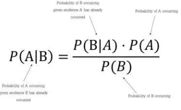
Fig 1 Naïve Bayes Formula
The word Bayes is added to the algorithm because it is taken form Bayes Theorem that is a conditional probability.
3.2 GENERAL REGRESSION NEURAL NETWORK:
The GRNN[8] is first introduced by Specht in 1991. Its related work is based on a neural network classifier. It is a four-layer network used in the regression task. The layer which comes first is called as load layer which gives some process line. The pattern sheet is a second surface that forms the basic covering and efficient for design instruction. The summation layer is a third layer that consists of pair nerve cell (ordinal and total summation). The fourth layer is dividing the value of sum somatic cell on the worth of the statistic cell. This network don’t require a repetitive presentation algorithm
Fig 2 General Regression Neural Network
In GRNN there is no need for back propagation. It uses the Gaussian function since it is high accuracy and estimation. It can handle noises in the input.
4
THEORETICAL
BACKGROUND
5981
5 METHODOLOGY
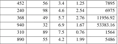
We have compared the results and accuracy of the prediction of the two algorithms Naive Bayes and GRNN.GRNN has been explained in the problem itself it is the efficient one and making the comparison of GRNN with Naïve Bayes. The dataset 40 records have been considered with attributes like UUCW, UAW, TCF, and EF.
TABLE 1
DATASET CONSISTING OF 40 RECORDS
UUCW UAW TC EF UCP
460 60 1.02 0.32 9008.64
550 30 20.1 0.62 205623
145 20 3.06 0.23 2041.02
360 50 5.04 0.65 58968
960 60 2.1 0.12 14515.2
750 40 6.1 0.24 43920
450 90 6.3 0.42 107163
550 50 5.1 0.35 49087.5
520 70 4.2 0.35 53508
620 50 3.04 0.93 87643.2
210 60 6.13 0.82 63335.16
620 30 5.31 0.12 11851.92
140 35 2.3 0.35 3944.5
320 65 6.1 0.24 30451.2
590 25 7.3 0.42 45223.5
360 45 6.7 0.63 68380.2
340 25 4.8 0.12 4896
420 35 5.08 0.24 17922.24
430 65 0.25 0.21 1467.375
310 60 1.3 0.36 8704.8
360 40 1.65 0.93 22096.8
320 90 1.48 0.37 15770.88
560 40 6.2 0.86 119436.8
254 50 9.3 0.54 63779.4
220 10 2.03 0.21 937.86
320 60 6.3 0.34 41126.4
620 30 5.6 0.25 26040
250 15 5.5 0.52 26000
230 18 3.6 0.43 41162.2
655 42 6.13 0.28 63353.61
201 66 7.6 0.24 11815.29
104 12 3.1 0.12 4869
950 52 5.8 0.22 1234
452 56 3.4 1.25 7895
240 98 4.6 2.54 6975
368 49 5.7 2.76 11956.92
940 32 6.9 1.67 53383.16
310 89 7.5 0.76 1564
890 55 4.2 1.99 5486
5.1 Code for the execution:
>mydata<-read.delim(file.choose(),sep=',',header= TRUE) >str(mydata)
>dim(mydata)
Making the partition of the dataset into testing and training. In the software R-studio, the dataset has been taken into the variable [mydata] and divided into the testing as well as training by the partition formula in the form of 30% and 70%. >tindex=sort(sample(nrow(mydata),nrow(mydata)*.7)) >mtraining=mydata[tindex,]
>mtesting=mydata[-tindex] >dim(mtraining)
>dim(mtesting)
Later on, the required Library e1071 has been installed and called for the usage of Naïve Bayes.
>install.packages(e1071) >library(e1071)
>NB<-naiveBayes(ef~.,data=mtraining) >print(NB)
>summary(NB)
>predNB1<-predict(NB,mtesting,type="class") >summary(predNB1)
>table(mtesting$ef,predNB1) >plot(predNB1)
But there is a problem in the prediction that is meant and says it is not suitable. With the help of the code executed in the software R-Studio which has proved that the Naïve Bayes is suitable for the prediction of the Effort for any software to be developed and it is proven that GRNN is the best for prediction.
6 RESULTS
5982 FIG 3 OUTPUT OF DIMENSIONS OF MYDATA
Input of Training and Testing
FIG 4 OUTPUT OF DIMENSIONS OF TRAINING AND TESTING
Installing package library
FIG 5 OUTPUT OF PACKAGE INSALLATION
Input: By using the formula of Naïve Bayes we are calculating the conditional probabilities .In this we are calling the Naive Bayes Algorithm.
FIG 6 PREDICTION OF NAÏVE BAYES
Input: Summary of Naïve Bayes
FIG 7 OUTPUT OF SUMMARY OF NB
FIG 8 SAYING THAT NB IS NOT SUITABLE
5983
6
CONCLUSION
The estimation of any software size and effort for any software product is a critical task to complete. UCP has played a major role in the estimation of the effort required to complete but later on, there are some drawbacks for the dynamic project estimation and differ from one to another. So these UCP can make to be calculated by using some soft computing techniques which predict the effort in the early stage itself. The analysis and comparative results of the algorithms like GRNN and Naïve Bayes have executed and concluded that Naïve Bayes is not at all suitable for this prediction rather in the review itself GRNN is suitable and efficient in the prediction of the estimating effort.
R
EFERENCES[1] G. Karner, "Resource estimation for objectory projects", Object. Syst., vol. 17, 1993.
[2] M. Azzeh, "Software cost estimation based on use case points for global software development", 5th Int. Conf. on Computer Science
and Information Technology (CSIT), pp. 214-218, 2013.
[3] B. Anda, H. Dreiem, D.I.K. Sjoberg et al., "Estimating software development effort based on use cases-experiences from industry", Proc. of the 4th Int. Conf. on the Unified Modeling Language Modeling Languages Concepts and Tools, pp. 487-502, 2001.
[4] D.F. Specht, "A general regression neural network", IEEE Trans. Neural Netw., vol. 2, no. 6, pp. 568-576, 1991.
[5] A.B. Nassif, L.F. Capretz, D. Ho, "Estimating software effort based on use case point model using sugeno fuzzy inference system", 23rd IEEE Int. Conf. on Tools with Artificial Intelligence, pp. 393-398, 2011
[6] M. Azzeh, A.B. Nassif, "Fuzzy model tree for early effort estimation", 12th Int. Conf. on Machine Learning and Applications (ICMLA), vol. 2, pp. 117-121, 2013.
[7] S.M. Satapathy, B.P. Acharya, S.K. Rath, "Early stage software effort
estimation using random forest technique based on use case points", IET Softw., vol. 10, no. 1, pp. 10-17, 2016
[8] Mohamm Adzzeh, Ali Bon Nassif, Shadi Banitaan, “comparative Analysis of soft computing Techniques for predicting Software Effort Based Use Case Points”,vol. 12,no . 1,2018
[9] Sabbineni Srinivas Rao, Inuganti Nava Sahitha, Godithi Sireesha, Palem Manoj"Evaluating Software System Reliability Using Architecture Based "International Journal of Intelligent Information Systems,2018; 7(1): 1-4,ISSN: 2328-7675 (Print); ISSN: 2328-7683 (Online).
[10] Dr.S.Srinivasa rao1,G.Moulika 2, Lalitkumar .G3 , D. Naga