Human Face Recognition Using Discriminant Analysis

159

Human Face Recognition Using Discriminant Analysis

Dr. Mohammed Saheb Mahdi Altaei

, Dua’a Ali Kareem

*

a,b_{Al-Nahrain University, College of Science, Computer Science Department, Baghdad, Iraq} a_{Email:[email protected]}

b_{Email:[email protected]}

Abstract

In the present research, a face recognition method is proposed based on the concept of linear discriminant analysis (LDA) method. The LDA requires input some of image models to analyze and discriminate them, the newly proposed idea is the use of a number of textural features instead of face image pixels to be input the LDA procedure. The employed textural features were ten, which are computed for each face image using the grey level co-occurrence matrix (GLCM) method. The proposed face recognition method consists of two phases: enrollment and recognition. The enrollment phase is responsible for collecting the features of each face image to be a comparable models stored in the database, while the recognition phase is responsible on comparing the extracted features of input unknown face with that stored in the database. The comparison results a number of percentage values, each refers to the similarity between the input unknown face with the models in the database. The recognition decision is then issued according to the comparison results. The results showed that the system performed the recognition test with a recognition percent of about 94%, whereas the validation test showed that the system performance was about 92%. Frequent practices showed that the behavior of the recognition is acceptable and it is enjoying with the ability to be improved.

Keywords: face recognition; LDA; GLCM.

1.Introduction

Identity recognition is used in wide range of applications including authentication, access control, face-based video indexing/browsing, and evenhuman-computer interaction/communication. Numerous techniques have been proposed for identity recognition depending on the used material [1]. The most confident used material is a part of human body, the science that deals with human body as unique key for identity recognition is the biometrics [2].

---

160

There are many different types of biometrics, including such long-established methods as fingerprints. Recently, biometrics based on speech recognition, gait (walking) recognition, and digital doggie (odor recognition) has been developed. Biometrics is currently a very active topic for research [3]. Face recognition systems identify people by their face images. Face recognition systems establish the presence of an authorized person rather than just checking whether a valid identification (ID) or key is being used or whether the user knows the secret personal identification numbers (Pins) or passwords [4].

Two issues are central to all face recognition algorithms, they are: the first is feature selection for face representation, while the second is the classification of a new face image based on the chosen feature representation [5].

2.Related works

There are a great deal of focus was granted to face recognition. Numerous approaches were developed in order to achieve more efficient techniques for serving applications in the field of interest. In the following, the most significant literatures are mentioned in details:

In 2003, Juwei and plataniotis established face recognition using kernel direct discriminant analysis algorithms, results indicate that the proposed methodology is able to achieve excellent performance with only a very small set of features being used, and its error rate is approximately 34% and 48% of those of two other commonly used kernel approaches, the kernel-pca (kpca) and the generalized discriminant analysis (gda) [6].

In 2011, Ali and Mary Face Recognition Based Wavelet-LDA Features And Skin Color Model, Experimental results demonstrate the higher degree performance of this algorithm

In 2013, Suman and kumar used linear discriminant analysis for face recognition , Here to identify an input test image, the projected test image is compared to each projected training, and the test image is identified as the closest training image. The experiments in this paper are performed with the ORL face database. The experimental results show that the correct recognition rate of this method is high [7].

3.Biometric system

161

4.Face recognition scenarios

A face recognition system is a computer application capable of identifying or verifying a person from a digital image or a video frames recorded by video source. Face recognition scenarios can be classified into two types: face verification (or authentication) and face identification (or recognition).

Face recognition approaches are either based on the use of images directly or the use of intermediate 3D models as Figure (2.2) shows. The first type that uses the image data are the techniques of interest, most of them depend on a representation of images that induces a vector space structure and requires dense correspondence. These approaches are called appearance-based or view-based approaches due to they represent an object in terms of several object views (raw intensity images). An image is considered as a high-dimensional vector, in which each point is represented in a high-dimensional vector space [ Xia98].

View-based approaches use statistical techniques to analyze the distribution of the object image vectors in the vector space, and derive an efficient and effective representation in the feature space according to different applications. There are three classical linear appearance-based classifiers are found, they are: principal component alalysis (PCA) [8], independent component analysis (ICA) [9], and linear descrimenant analysis (LDA) as Figure (1) shows [10].

Figure 1: Face recognition approaches [10].

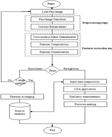
5.Proposed face recognition

The concept of multistage processing and features extraction has been used to design the proposed face recognition method. It is claimed that these stages can beneficially be combined to establish a fast and efficient face recognition application.

162

whereas three steps are found in features extraction stage includes: cooccurrence matrix determination, features computation, and features normalization. Then, LDA is applied on the features array to indicate the discriminant factors. Last stage is a comparison based on the discriminant factor is carried out between the results of LDA depending on the training models of each class found in the database, the result of the comparison will determine the similarity measure between the considered face images. These similarity scores are then numerically ranked in a descending order. The percentage of times that the highest similarity score is the correct match for all individuals is referred to as the top match score. Accordingly, the match score help to make a face recognition decision. More details about each stage are given in the following sections:

Figure 2: Generic structure of proposed face recognition method.

5.1 Preprocessing stage

The preprocessing is a primary stage aims at preparing face image for highlighting the image cues that leads to estimate recognizable face features. The preprocessing stage includes two steps, they are: image transformation and contrast enhancement. The following subsections explain more details about each step:

a.Image transformation

Image transformation uses the equation of transforming the three components of the color image RGB into the intensity-chrominance components YIQ. Actually, just the first component that refers to the intensity is useful in current step that given in the following relation:

𝐺𝐺= 0.299 ×𝑓𝑓𝑅𝑅+ 0.587 ×𝑓𝑓𝐺𝐺+ 0.114 ×𝑓𝑓𝐵𝐵 (1),[ 11]

Where, G is the intensity component of the colored image f, while fR, fG, and fB are the color components that

163

image cue that carried by the three color components of the face image along the visible spectrum, also the intensity image will includes all the image features that may be useful for face recognition task

b. Contrast enhancement

Image enhancement includes using linear fitting model to improve the contrast of the face image. By assuming that the measured minimum and maximum values of the spectral intensity image G are Gmin and Gmax frequently,

and the intended minimum and maximum values of enhanced intensity image E are Emin and Emax frequently,

then the enhanced image E is related to the spectral intensity image G by the following linear relationship:

𝐸𝐸=𝑎𝑎×𝐺𝐺+𝑏𝑏 (2)

Where, a and b are the coefficients of the linear fitting model between G and E. the substitution of both Gmin and

Gmax that measured from the G image and the known values of Emin and Emax in eq.(3), one can gets the

following two relations that containing just two unknowns a and b:

𝐸𝐸𝑚𝑚𝑚𝑚𝑚𝑚=𝑎𝑎×𝐺𝐺𝑚𝑚𝑚𝑚𝑚𝑚+𝑏𝑏 (3)

𝐸𝐸𝑚𝑚𝑚𝑚𝑚𝑚=𝑎𝑎×𝐺𝐺𝑚𝑚𝑚𝑚𝑚𝑚+𝑏𝑏 (4)

The use of equations (3 and 4) as a set of two equations with two variables enables to estimate the two unknown variable values of the linear fitting coefficients a and b by the substitution as follows:

𝑎𝑎= (𝐺𝐺𝑚𝑚𝑚𝑚𝑚𝑚− 𝐺𝐺𝑚𝑚𝑚𝑚𝑚𝑚)/(𝐸𝐸𝑚𝑚𝑚𝑚𝑚𝑚− 𝐸𝐸𝑚𝑚𝑚𝑚𝑚𝑚) (5)

𝑏𝑏= (𝐺𝐺𝑚𝑚𝑚𝑚𝑚𝑚×𝐸𝐸𝑚𝑚𝑚𝑚𝑚𝑚− 𝐺𝐺𝑚𝑚𝑚𝑚𝑚𝑚×𝐸𝐸𝑚𝑚𝑚𝑚𝑚𝑚)/(𝐸𝐸𝑚𝑚𝑚𝑚𝑚𝑚− 𝐸𝐸𝑚𝑚𝑚𝑚𝑚𝑚) … (6)

The determination of both linear fitting coefficients a and b gives the ability to compute all the pixels of the enhanced image according to eq.(2).

5.2 Features extraction

This stage includes three steps within for achieving the identity features that the enhanced face image belong to. These three stages are: co-occurrence matrix determination, features computations, and features normalization. More details about each step are given in the following subsections:

a.Co-occurrence matrix determination

This step is applied on the enhanced image. Such that, the grey levels of the enhanced image are firstly quantized into few level values (Lg), e.g. five levels, each level represents a specific range of greys in the

164

Then, the frequency of each element in Q array is computed by counting the probable transitions happen between each two pointers in Q array to be stored in newly created squared array is the frequency array (F) of size Lg×Lg. The probability of appearing each pixel in the enhanced image is stored in P array of same size as F

that can be estimated by dividing each element of F by the total number of transitions, the total number (TT) of

transition is determined by the following relation:

𝑇𝑇𝑇𝑇=𝐿𝐿𝑔𝑔−1 ×𝐿𝐿𝑔𝑔−1 (7)

b.Features computations

This stage includes computing the ten textural features, the computations of these equations depend on the accuracy of determining the probability P of appearing each pixel in the enhanced image. The different distribution of spectral intensity in each face image of different identity produces different features and leads to different probable spectral distribution of pixels at the image space. Different location of pixels between different face images is almost leading to different textural features belong to different face images, whereas it is normally to find the textural features are similar for same face image even with different samples. In general, the computed features are stored in features vector V of length is equal to the number of features (NF), which is split

into NS×NI sub vectors, each refers to features of one sample in the dataset.

C. Features normalization

Due to the used textural features belong to different conceptual basis; the equations of their computations are also different. This cause to produce a result is ling in different numerical range according to each feature. The use of same computed feature value may cause to bias the recognition decision into some features of great values, whereas the activity of the low valued features will be relatively lower. Therefore, it should be equalized the contribution of all the used features in producing the recognition decision.

This is can be carried out by normalizing features values to be within the range from -1 to 1, this require to find out the maximum 𝑉𝑉_𝑗𝑗𝑚𝑚𝑚𝑚𝑚𝑚 and minimum 𝑉𝑉_𝑗𝑗𝑚𝑚𝑚𝑚𝑚𝑚 values of a jth feature Vj for all used samples in the dataset, and then

use the following relationship to normalize this feature.

𝑁𝑁𝑗𝑗= [2 × (𝑉𝑉𝑗𝑗−𝑉𝑉𝑗𝑗

𝑚𝑚𝑚𝑚𝑚𝑚₎

(𝑉𝑉_𝑗𝑗𝑚𝑚𝑚𝑚𝑚𝑚−𝑉𝑉_𝑗𝑗𝑚𝑚𝑚𝑚𝑚𝑚)]−1 (8)

Where, j is pointer refers to the feature serial in the features vector, Ni refers to the ith normalized feature in the

features vector.

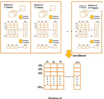
6.Enrollment phase

165

their features and then the average of each feature is stored in A with same index of that feature. The collection of all averaging feature of NI identities are stored in D, which is a database represented by a two

dimensional array of size NF×NI, Figure (3) shows the process features averaging that applied on the dataset

image to create the database array D.

Figure 3: The enrollment phase workflow.

7.Recognition phase

The recognition phase aims to issue a recognition decision based on quantitative comparison between the features of the query face image and that ones found in the database. The results of the comparisons indicate how the query unknown face is similar (close) to the face samples in the database. It is expected that there is at least one similar sample when the query face is predefined in the codebook, and there is a high recognition score. Otherwise the recognition scores that come from the estimated similarities are dispersed between other samples, and there is no highly score attended. There is three interested stages are adopted to make accurate recognition decision; the first aims to prepare the entry data of the adopted LDA method, the second is implementing the LDA algorithm using the prepared database, and the third one is concerned with estimating the percent of similarities between the query face and the samples of the database, and the result will be a similarity percentage indicates the a unique recognition decision. More details about the recognition steps are given in the following subsections:

7.1 Data composition

The recognition face deals with the features vector of unknown input image and that of the face samples found in database array D. It is firstly takes the contents of D and stored it in a newly created array X, which is the LDA input data array. The size of X array is same as D with additional last column represents the features vector of the input unknown face image, i.e. NF× NI+1

166

The newly suggested idea is the use of features vector instead of pixel values that arranged in one column of face image when constructing the input data of the LDA. Therefore, LDA algorithm is applied on the features array X to estimate the relational vector R that contains NI+1 elements, each represents the relation of feature of

same index with the corresponding features in the database.

7.3 Similarity measurement

The similarity measure (Si) can be computed by the difference between the last value of R (i.e. RNI+1) and its

previous values as follows:

𝑆𝑆𝑚𝑚=�1−_∑|𝑅𝑅𝑚𝑚_|−𝑅𝑅_𝑅𝑅 𝑁𝑁𝑁𝑁+1|

𝑚𝑚−𝑅𝑅𝑁𝑁𝑁𝑁+1| 𝑁𝑁𝑁𝑁

𝑚𝑚=1 �× 100% (9)

In such case, Si gives the amount of similarity between the last element in the vector R that belongs to the input

unknown face image and other elements of the vector R that belong to known identities stored in the database. The recognition decision depends refers to database identity of the most similarity percent.

8.Result and discussion

The development of face recognition brings about an easy way to establish useful applications for face based authentication methods. Consequently, the behavioral performance of such methods is examined using validation and assurance techniques. In the present work, there are two considered paths; enrollment and recognition. The enrollment is useful to indicate the basic characterstics of each face image that represented by some specified statistical features, while the recognition uses the same features to produce the final recognition decisions in terms of enrollment results. Results validation is carried out for assurance purpose.

The validation includes a clear picture about the performance of the used algorithms mentioned in the previous chapter. Also, there is a detailed explanation related to the results achieved through implementing each stage in the proposed LDA based face recognition method. The results are presented in figures and tables including the final percentage of recognition. Then, quantitative and qualitative analysis is estimated to evaluate the performance of the proposed recognition method. Moreover, the implementation of the proposed method was designed by C# programming language that executed under Windows 8 operating system. The dedicated classification method was designed to include package of preprocessing and post processing that mentioned previously, also it shows pretty interface for displaying the results of each stage individually. The following sections show more details about the results and discussions of the employed method.

9.Face image dataset

167

The used dataset of face image are downloaded from CASIA web site, that provides huge database of images, each is collected at specific stuations for a specific subject. This used CASIA dataset consists of 100 face in total (NI=100), including 57 males and 43 females. All face images are 24 bit per pixel are saved in colored

JPEG file format, which are recorded under visible illumination with spatial resolution 256*256. There are about 10 sample images are available for each face in the collected dataset, the enrolled database is depends on using only five samples (NS=5) for each face, same these five samples are also used for testing the proposed

mthod, whereas the other five samples are used to implement the validation and generalization test.

In general, different characteristics of the face image subsets make it possible to study specific research issues of face recognition, such as robustness of face recognition against illumination changes or face allocation that can affect the results of face recognition. Figure (4) shows some samples of the used CASIA face dataset.

Figure 4: Some image samples for different faces in the used dataset.

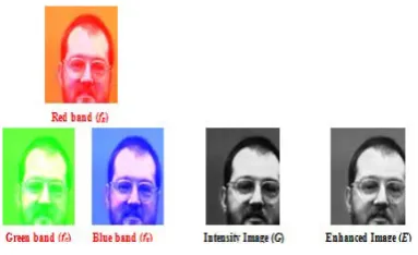
Image preprocessing is an image enhancement stage that impacts the grey distribution and histogram of the image. It is applied on the three color bands (red, green, and blue) of the image to be converted into one enhanced intensity band is suited for machine based analysis. Then, the grey levels of the intensity image are stretched along the full grey scale, which leads to make image details to be more clearly shown. Figure (5) shows the three color components of one face image sample and its corresponding intensity and transformed images. Whereas, Figure (6) shows the histogram stretching of the intensity image.

168

Figure 6: Histogram enhancement of preprocessing stage.

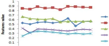
10. Features extraction results

The used features are ten textural ones (NF=10). Figure (7) shows the behaviors of normalized values of the ten

features (features set) for just five different image samples of same face. Also, Figure (8) shows the behavior of normalized values of the features set for five different image samples of different faces. In general, there are 500 features set belong to the 100 face image found in the used dataset, each contributed with 5 samples. More practice showed there are some stability is shown in the behavior of featires set for same face image with different image samples, and fewer irregularities are shown in the behavior of each feature that belong to different sample of same face image

Figure 7: Behaviors of normalized extracted features set of five different samples belong to different face images,

Figure 8: Behaviors of normalized extracted features set of five different samples belong to same face image,

11. Enrollment results

169

average is almost same as features but not identical. Therefore, this is the reason that make the recognition score not to be full percent. Figure (10) shows five average behaviors in the database belong to five different samples of different face images.

Figure 9: Behaviors of normalized extracted features set of five different samples belong to same face image,

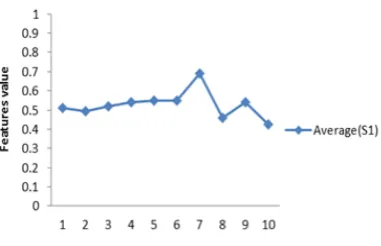
Figure 10: Behaviors of five averages in the database belong to five different samples of different face images.

12. Recognition results

The results of the recognition are a set of percent scores equal to the number of the input face images (i.e. NI

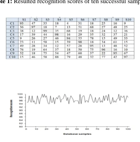
scores), each represents the similarity percent of the input unknown face image with that stored in the database. Table (1) presents the recognition scores for ten runs, each for one sample from that found in the database.

The rows in the table contains ten test samples of input face images from that used to establish the database, while the columns represent the corresponding classes that its average features are recorded in the database. It is shown that the scores lies on the diagonal is high in comparison with others, these diagonal scores describe the similarity between the input image and the samples of the database of same class.

170

Table 1: Resulted recognition scores of ten successful samples.

Figure 11: Average of the resulted recognition score of samples found in the dataset.

In spit of more fluctuations are found in the behavior of the average scores when using all the face samples found in the dataset, the mean value of them is still stable and near the percent 96%. Also, it is shown that the change rate of fluctuated average behavior progresses horizontally and there is no decay may occure with increasing the size of dataset. It is found that the range of the flections is about ±2%, which is small range in comparison with the high values of recognition score, such that, this type of fluctuation can be regarded as acceptable

13. Recognition validation

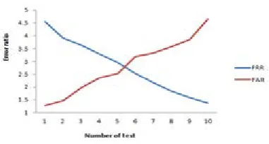
The recognition validation is an important test based on using five face image samples for each regarded class that are not previously used in the enrollment stage to establish the database. In this test, both FRR and FAR are computed to evaluate the performance of the proposed method, which leads to indicates expected error ratio (EER) and the percent of performance accuracy. The EER is the average value of the two types of erroes:

FRR and FAR. The validation of recognition performance is tested on two face image samples for each class to find the performance accuracy against the EER where the FAR and FRR are approximately equal in the ROC curve. Table (2) lists the computed average error values of ten test run for the five recognition samples against their FRR and FAR ratios, Figure (12) shows the behavior of FRR and FAR that given in Table (2). Whereas, Table (3) lists the computed average error values of ten test run for the two validation samples against their FRR and FAR ratios, Figure (13) shows the behavior of FRR and FAR that given in Table (3).

171

Table 2: Resulted average error of the recognition test.

Figure 12: ROC curve of FRR and FAR for recognition process..

Table 3: Resulted average error of the validation test

172

14. Conclusions

Throughout the implementation of the present work, a number of conclusions have been achieved based on the practical results. The following statements summarize the most important ones:

1. The behaviors of the textural features were monotonic with the variation of dataset size, and the use of more samples does not change the performance of the proposed method.

2. the enhanced images have more contrast than the original image since more embedded colors may found in the original image are appeared after enhancement. Sharp edges and clear extended regions are very useful to describe the face in terms of numerical features

3. there are some stability is shown in the behavior of features set for same face image with different image samples, and fewer irregularities are shown in the behavior of each feature that belong to different sample of same face image.

4. In spit of more fluctuations are found in the behavior of the average scores when using all the face samples found in the dataset, the mean value of them is still stable and near the percent 96%.

5. Throughout test of the recognition, it is shown that the best operating point is occurred when the FAR and FRR are approximately equal at EER of about 2.864% that make the performance accuracy to be 94.272%. While the test of validation gives EER equal to 2.780% that make the performance accuracy about 94.439%.

15. Suggestions for Future Work

1.The use of more features will lead to increase the recognition score and even the accuracy of the proposed method performance.

2.The faces can be recogntion by the features extracted from the video.

3.Another form of classifiers can be used rather than LDA for example neural network, support vector machine ..etc.

Acknowledgment

Great thanks to to my supervisor Dr. Mohammed S. Altaei who gave us all the supporting, helpfulness, assistance, encouragement, valuable advice, for giving me the major steps to go on for exploring the subject, sharing with me the ideas in my research, and discuss the points that I left they are important. Grateful thanks are due to staff of Computer Science Department for supportion. Also, sincere thanks to our friends those give advises.

References

173

[2] David Lott, April 2015, “IMPROVING CUSTOMER AUTHENTICATION”

[3] John Wiley & Sons “Information Security Principles And Practice” San Jose State University

[4] Divyarajsinh N. Parmar, Brijesh B. Mehta 2013 “Face Recognition Methods & Applications” Int.J.Computer Technology & Applications,Vol 4.

[5] Guo-Dong Guo, Hong-Jiang Zhang, and Stan Z. Li, 2001 IEEE ,“Pairwise Face Recognition”

[6] Juwei Lu, Konstantinos N. Plataniotis,and Anastasios N. Venetsanopoulos, 2003,” Face Recognition Using Kernel Direct Discriminant Analysis Algorithms” IEEE TRANSACTIONS ON NEURAL NETWORKS, 14(1).

[7] Suman Kumar Bhattacharyya And Kumar Rahul, 2013, “Face Recognition By Linear Discriminant Analysis” International Journal Of Communication Network Security, 2(2).

[8] Matthew Turk and Alex Pentland, 1998 “Eigenfaces for Recognition” Journal of Cognitive Neuroscience, 3(1).

[9] Marian Stewart Bartletta, H. Martin and Terrence Sejnowski, 1998, “Independent component representations for face recognition”.

[10] Peter N. Belhumeur Joao P. Hespanha David and J. Kriegman, 1997 “Eigen faces Vs. Fisher faces: Recognition Using Class Speci_C Linear Projection” IEE Trans. On Pami.