Two Activation Function Wavelet Network for the Identification of Functions with High Nonlinearity

(1)

Two Activation Function Wavelet Network for the

Identification of Functions with High

Nonlinearity

Wisam Khalid Abdulkader

Abstract-- The integration of wavelet theory into soft computing have recently attracted great interest. The first real integration of wavelet into soft computing led to the development of wavelet-networks. In this work, a robust Two Activation Function Wavelet Network (TAFWN) is proposed for the identification of functions with high nonlinearity. The TAFWN is further trained by the least mean squares (LMS) to minimize the mean-squared error. Simulation results are demonstrated to validate the identification ability and efficiency of the proposed network.

Index Terms-- Wavelet Network, Neural network, Identification.

I. INTRODUCTION

A neural network is an interconnected network of simple processing elements, e.g. scaling and filtering. The processing elements interact along paths of variable connection strengths which when suitably adapted can collectively produce complex overall desired behavior. Obviously neural networks are well suited to solving the same types of problems as the human’s brain. Particularly, neural networks excel at recognition, identification, and classification types of problems [1]. Neural networks have been applied very successfully in the identification and control of dynamic systems. The universal approximation capabilities of the multilayer perceptron (the backpropogation algorithm) make it a popular choice for modeling nonlinear systems and for implementing general-purpose nonlinear controllers [2]. Neural networks have been employed successfully in adaptive control system design problems of nonlinear systems, but there are still some difficulties in neural network-based Wisam

adaptive control designs. The basis functions are generally not orthogonal or redundant; i.e., the network representation is not unique and is probably not the most efficient one. Furthermore, the convergence of neural networks may not be guaranteed. Even when it exhibits a good convergence rate, the training procedure may still be trapped in some local minima, depending on the initial settings.

Wisam Khalid Abdulkader University of Kufa, Iraq

[email protected]

In addition, approximation errors and external disturbances cannot be efficiently attenuated. Hence, performance and even stability may not be guaranteed. By combining the idea of neural networks and the merits of wavelets, a wavelet network was developed and it's considered as a special case of a RBF network [3]. Wavelet networks can in some situations be an attractive alternative to other neural networks such as sigmoid feed-forward and Radial Basis Function (RBF) networks [4]. In this paper, Two Activation Function Wavelet Network algorithm is proposed. It introduces an identification model of Two Activation Function Wavelet Network and compares simulations of Wavenet and Two Activation Function Wavelet Network algorithms for their learning abilities to identify single variable nonlinear functions.

II. NEURAL NETWORK ADAPTIVE WAVELETS (Wavenets)

Wavelet neural networks (WN) are feed-forward neural networks using wavelets as activation function. WN have been used in classification and identification problems with some success. In wavelet networks, both the position and the dilation of the wavelets are optimized besides the weights [5]. WNs have recently attracted great interest, because of their advantages over RBF networks as they are universal approximators but achieve faster convergence and are capable of dealing with large dimension and non-stationary signals. In addition, WNs are generalized RBF networks [6]. WNs have a wide variety of application areas, like speech recognition and digital communication. They were also applied in robot applications where robot kinematics is a continuous function and operates in a bounded range [7].

(2)

2(t). Accordingly, there are two scaling filters and two wavelet filters.

IV. THE TWO ACTIVATION FUNCTION WAVELET NETWORK ALGORITHM The TAFWN architecture approximates any desired signal

)

(

t

y

by generalizing a linear combination of two set of daughter wavelets

h

₁_,_a_,_b

(

t

)

and

_h

₂_,_a_,_b

₍

_t

₎

, where the daughter wavelets

h

₁_,_a_,_b

(

t

)

and

_h

₂_,_a_,_b

₍

_t

₎

are generated by dilation,

a

, and translation,

b

, from two mother wavelets

)

(

)

(

2 1



and

h



h

, where

a

b

t







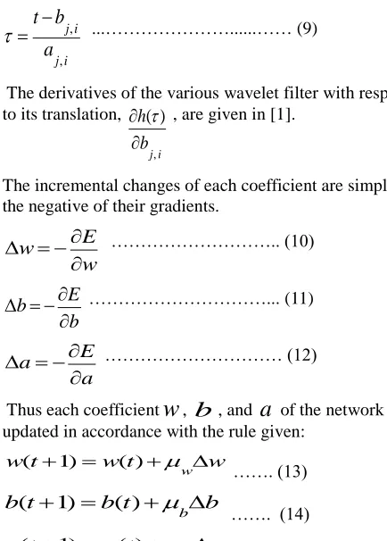
. The network architecture

is shown in figure (1):

)

(

)

(

1 , , 1

a

b

t

h

t

h

ab





………….… (1)

)

(

)

(

2 , , 2

a

b

t

h

t

h

ab





…..………… (2)

where

a

: Dilation factor, with

a

> 0.

b

: Translation factor.

:

t

Signal time interval

A TAFWN is a 3-layers feed forward neural network. First the TAFWN parameters, dilation a's, translation b's, and weight w's should be initialized, and the desired sets of data, the input signal x(t), the desired output (target)

y(t), the number of scaling functions p (p=2 in this work) and the number of wavelons k are given.

Assuming that the network output function satisfies the admissibility condition and the network sufficiently approximates the target. The approximated signal of the network

_y

ˆ

₍

_t

₎

can be represented by equation:







  k

i j i a_j _i b_j _i p

j

w

h

t

x

t

y

1 , _, , _,

1

(

)

(

)

(

ˆ

……. (3) where

x(t) is the input signal.

i j

w

, is the weight coefficients between hidden and output layers.

j=1,2,…, p. p=2: a number of scaling functions.

i=1,2,…, k. k is a number of wavelons.

i j b i j a

h

, , ,

is a two set of daughter wavelets generated

from two mother wavelets

₍

_),

₍

₎

2

1

t

h

t

h

as in equations

(1) and (2) respectively.

Similar to WN, after constructing the initial TAFWN and after calculating output signal of the network, the training of TAFWN starts. It is further trained by the gradient descent algorithms like least mean squares (LMS) to minimize the mean-squared error. During learning, the parameters of the network are optimized

.

The TAFWN parameters

i j

w

_, ,

i j

a

_, , and

i j

b

, can be optimized in the LMS algorithm by minimizing a cost function or the energy function,

E

, over all function interval. The energy function is defined by equations (4) and (5),

_y

₍

_t

₎

is the desired output (target) and

_y

ˆ

₍

_t

₎

is the actual output signal of TAFWN.

   T t t e E 1 2 ) ( 2

1 ……….… (4)

_ 





T t

t

y

t

y

E

1 2

))

(

ˆ

)

(

2

1

……….(5)

where

T

is the total interval of function,

y

(

t

)

is the desired output (target) and

_y

ˆ

₍

_t

₎

is the actual output signal of WN.

To minimize E the method of steepest descent is used, which requires the gradients

i j

w

E

,



, i j

a

E

,



, and

i j

b

E

,



for

updating the incremental changes to each particular parameter

i j

w_, ,

a

_j_,_i, and

b

_j_,_i, respectively. The gradients of

E

are:

i j w E ,  







 T t

t

x

h

t

e

1

)

(

)

(

)

(



……..…….(6)

i j b E ,  

_







 T t i j i j

b

h

w

t

x

t

e

1 , ,

)

(

)

(

)

(



…(7)

(3)

i j i j

a

b

t

, ,







...………...…… (9)

The derivatives of the various wavelet filter with respect to its translation,

i j b h , ) ( 





, are given in [1].

The incremental changes of each coefficient are simply the negative of their gradients.

w

E

w









……….. (10)

b

E

b









………... (11)

a

E

a









……… (12)

Thus each coefficient

w

,

b

, and

a

of the network is updated in accordance with the rule given:

w t w t w w  

1) ( )



( ……. (13)

b

t

b

t

b









1 )

(

)



(

……. (14)

a t

a( 1) ( )



_a

...…… (15)

Where



is the fixed learning rate parameter [1].

At each iteration, the network parameters are modified using the gradient descent algorithm till one of the stopping conditions described is satisfied.

The training algorithm of the proposed two activation function wavelet network consists of the following six steps:

1. Initialize TAFWN parameters, dilation a's, translation b's, and weight w's, p=2, two mother wavelets filters

                            i a i b t i a i b t h h 2 1 ,

, the desired sets of data, the

input signal x(t), the desired output (target) y(t), and the number of wavelons k are given.

2. Set: the number of trainings, iter = 0, the incremental

changes of each coefficient,

(



w

,



a

,



b

)

=0, and the initial square error, _₀_.₅

iter

E

3. Calculate the approximated signal of the network

)

(

ˆ

t

y

using equation (3).

4. Calculate the gradients of each coefficient using equations (4), (5), (6) and calculate the coefficients incremental changes which are the negative of their gradients.

5. Choose a constant 0.01 ≤



≤1 and calculate the new coefficients 1  iter

w

, 1  iter

b

, and

1



iter

a

of the network

in accordance with the rules given in equations (13), (14) and (15).

6. Calculate the square error

1



iter

E

using equation (5).

If

1



iter

E

is small enough, then the training is good and the algorithm is stopped. Otherwise, set iter = iter + 1 and go to (3).

V. TAFWNIDENTIFICATIONMODEL

Figure (2) shows the TAFWN Identification Model configuration of a nonlinear function approximation and its essential features. The function f(x) and the two wavelet filters are driven by the same input signal. The wavelet filters acting on an input sequence x(n) to produce an output signal y(n). The output signal d(n) supplies the desired output signal for the wavelet filter that approximates the nonlinear function characteristic.

The filter is designed so that the output should approximate a training signal or desired output d(n). The estimation error e(n), which is used for controlling the filter coefficients, is the difference between the desired output signal and the actual output signal of the adaptive system.

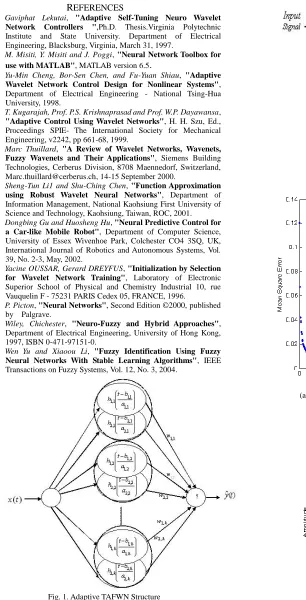
VI. SIMULATION CONFIGURATION AND RESULTS

The TAFWN algorithm, with one hidden layer of twenty [20 Morlet, 20 Slog1] wavelons in the hidden neurons (k = 20) and fixed learning rate of 1 is implemented to identify this hard nonlinear function:

)

9 .

0 (

4 sin(

)

6 .

0 (

3 sin(

)

1 (

0025

2 )

(









21



2



3(0.5)



2

x

e

x

e

x

f

x



x



………... (16)

for x



[ 0,1] , where the interval width is 0.01 [8].

Initial w's and dilations a's are set to 0 and 7 respectively. b's are spaced equally apart throughout the training data. The simulation result shown in Figure (3- a, b, c). Figure (3-a) shows the MSE against the number of iterations for off-line training of the network. Figure (3-b) illustrates the performance results of the network identifying the function given above.

The trained TAFWN is tested using an input sequence with interval width of 0.001 instead of 0.01 without changing the coefficients (k, a's, b's, and w's) produced in training. With MSE equals to 0.0041 the approximated signal is obtained as shown in figure (4).

VII. WAVELET NETWORK vs. TAFWN

In the previous sections, TAFWN Networks are proven to be, as well as many other neural paradigms, a specific case of the generic paradigm named RBF Networks.

(4)

simulations of Wavenets algorithm and the TAFW Network algorithm will be investigated and compared for their learning abilities to identify the nonlinear functions as it is presented in the following two examples. This section will confirm this idea by providing several observations derived from the results of the MATLAB simulations.

RESULTS

Simulations of Wavenets algorithm and the TAFW Network algorithm is compared for their learning abilities to identify the piecewise defined nonlinear function of a single variable given by:

-2.186x-12.864 for x



[-10,-2]

f(x )= 4.246x for x



[-2 , 0]

10 _e

0.05x0.5

_{sin((0.03x+0.7)x) for x}



_{[ 0,10]}

… …….. (17)

where the interval width is 0.1.

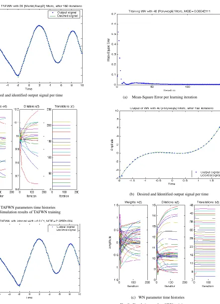
Figures (5-a) and (6-a) show the MSE against the number of iterations for off-line training of each network. Figures (5-b) and (6-b) illustrate the performance results of the two networks

The WN with one hidden layer of forty [40 Morlet] wavelons in the hidden neurons (k = 40). All learning rate parameters for weights, dilations, and translations are fixed at 0.01 and initial weights w's and dilations a's are set to 0 and 10, respectively. Initial translation parameters b's are spaced equally apart throughout the training data to provide non-overlapping partitions throughout the neighboring intervals.

TAFWN with one hidden layer of twenty [20 Morlet, 20 Rasp2] wavelons in the hidden neurons (k = 20), and fixed learning rate of 0.01. Initial weights w's and dilations a's are set to 0 and 10, respectively. Initial translation parameters b's are also spaced equally apart throughout the training data. Note, that there are no particular reasons governing the choice of these parameters. These parameters were obtained from the experience of many simulations that were found to be efficient.

In figure (5-a), which represents the WN training, it can be noted that the obtained MSE equal to 0.0011 in 150 iterations. Figure (6-a) show that by using TAFWN training the MSE value equal to 1.6640e-004 also in 150 iterations, while the MSE equal to 0.0011 at only 8 iterations. That’s proving how the identification property of TAFWN is strikingly improved and the training speed is greatly increased over wavelet network. Table (1) gives a comparison between these two identifier network training in number of iterations, Time, and MSE value.

The trained TAFWN is tested using an input sequence with interval width of 0.01 instead of 0.1 without changing the

coefficients (k, a's, b's, and w's) which have been produced from training TAFWN. With MSE equals to 2.5237e-004 the approximated signal of 0.01 interval widths is obtained with respect to the desired signal as shown in figure (7).

By using both WN and the proposed TAFWN to approximate another nonlinear function given in equation (18) as shown in figures (8) and (9), it can be noted how the TAFWN training is readier than WN training. Table (2) gives a comparison between the training (number of iterations, Time, and MSE value) of these two networks:

x

f

(

)



3



0 .

3

2



0 .

4

_{…….…. (18)}

For x



[-2, 2], where the interval width is 0.1.

The WN with one hidden layer of forty [40 Polywog5] wavelons in the hidden neurons (k = 40), all learning rate parameters for weights, dilations, and translations are fixed at 0.02. All initial weights w's and dilations a's are set to 0 and 10, respectively. Initial translation parameters b's are spaced equally apart throughout the training data to provide non-overlapping partitions throughout the neighboring intervals.

The TAFWN with one hidden layer of twenty [20 Rasp1, 20 Polywog5] wavelons in the hidden neurons (k = 20), and fixed learning rate of 0.01. All initial weights w's and dilations a's are set to 0 and 8, respectively. Initial translation parameters b's are spaced equally apart throughout the training data.

The trained TAFWN is tested using an input sequence with interval width of 0.01 instead of 0.1 without changing the coefficients (k, a's, b's, and w's) which have been produced from training TAFWN. With MSE equals to 1.3987e-005 the approximated signal of 0.01 interval widths is obtained with respect to the desired signal as shown in figure (10).

VIII. CONCLUSIONS

An advanced wavelet network, called Two Activation Function Wavelet Network is proposed as an interesting alternative to wavelet networks. This technique absorbs the advantage of high resolution of wavelets and the advantages of learning and feed-forward of neural networks. It is shown how the identification property of wavelet neural network is strikingly improved and the training speed is greatly increased through the proposed Two Activation Function Wavelet Network (TAFWN).

Several algorithms for function identification are designed, implemented, and tested using Matlab tool.

(5)

REFERENCES

[1] Gaviphat Lekutai, "Adaptive Self-Tuning Neuro Wavelet Network Controllers ",Ph.D. Thesis.Virginia Polytechnic Institute and State University. Department of Electrical Engineering, Blacksburg, Virginia, March 31, 1997.

[2] M. Misiti, Y. Misiti and J. Poggi, "Neural Network Toolbox for use with MATLAB", MATLAB version 6.5.

[3] Yu-Min Cheng, Bor-Sen Chen, and Fu-Yuan Shiau, "Adaptive Wavelet Network Control Design for Nonlinear Systems", Department of Electrical Engineering - National Tsing-Hua University, 1998.

[4] T. Kugarajah, Prof. P.S. Krishnaprasad and Prof. W.P. Dayawansa, "Adaptive Control Using Wavelet Networks", H. H. Szu, Ed., Proceedings SPIE- The International Society for Mechanical Engineering, v2242, pp 661-68, 1999.

[5] Marc Thuillard, "A Review of Wavelet Networks, Wavenets, Fuzzy Wavenets and Their Applications", Siemens Building Technologies, Cerberus Division, 8708 Maennedorf, Switzerland, [email protected], 14-15 September 2000.

[6] Sheng-Tun Li1 and Shu-Ching Chen, "Function Approximation using Robust Wavelet Neural Networks", Department of Information Management, National Kaohsiung First University of Science and Technology, Kaohsiung, Taiwan, ROC, 2001. [7] Dongbing Gu and Huosheng Hu, "Neural Predictive Control for

a Car-like Mobile Robot", Department of Computer Science, University of Essex Wivenhoe Park, Colchester CO4 3SQ, UK, International Journal of Robotics and Autonomous Systems, Vol. 39, No. 2-3, May, 2002.

[8] Yacine OUSSAR, Gerard DREYFUS, "Initialization by Selection for Wavelet Network Training", Laboratory of Electronic Superior School of Physical and Chemistry Industrial 10, rue Vauquelin F - 75231 PARIS Cedex 05, FRANCE, 1996.

[10] Wiley, Chichester, "Neuro-Fuzzy and Hybrid Approaches", Department of Electrical Engineering, University of Hong Kong, 1997, ISBN 0-471-97151-0.

[11] Wen Yu and Xiaoou Li, "Fuzzy Identification Using Fuzzy Neural Networks With Stable Learning Algorithms", IEEE Transactions on Fuzzy Systems, Vol. 12, No. 3, 2004.

Fig. 1. Adaptive TAFWN Structure

Fig. 2. TAFWN Identification Model

(a) Mean-Square Error per learning iteration

(6)

(c) TAFWN parameter time histories Fig. 3. Simulation results of TAFWN training

Fig. 4. Output signal of trained TAFWN

(b) Desired and Identified output signal per time

(c) WN parameters time histories Fig. 5. Simulation results of WN training

(7)

(b) Desired and identified output signal per time

(c) TAFWN parameters time histories Fig. 6. Simulation results of TAFWN training

Fig. 7. Output signal of trained TAFWN

(b) Desired and Identified output signal per time

(c) WN parameter time histories

Fig. 8. Simulation results of WN training

(8)

(b) Mean-Square Error per learning iteration

(c) TAFWN parameter time histories

Fig. 9. Simulation results of TAFWN training.

Fig. 10. Output signal of trainedTAFWN

TABLE I

Comparisons between WN and TAFWN of their learning abilities

Network type

No. of iterations

Time

MSE value

TAFWN

150 131 sec

0.00016640

WN

150 135 sec

0.0011

TAFWN

15 13 sec

0.00057256

WN

15 14 sec

0.0049

TABLE II

Comparisons between WN and TAFWN of their learning abilities

Network type

No. of iterations Time

MSE value

TAFWN

150 28 sec

0.000017641

WN

150 26 sec

0.00042111

TAFWN

50 10 sec

0.000021527