Abstract--This paper investigates the suitability of Delay Vector Variance (DVV) algorithm in determining the presence of non-linear and stochastic nature of time series both in the presence and absence of chaos. A differential entropy based method is used to find the optimum embedding dimension and time lag which are needed to represent the time series in phase space. Results obtained from the simulation indicate that the DVV method gives quantitative and easy to interpret output to characterize the underlying times series in terms of non-linear and stochastic nature.
Index Term-- Delay Vector Variance (DVV), Entropy Ratio(ER), Nonlinearity, Phase S pace.
I. INT RODUCT ION
Atime series becomes chaotic due to the presence of determinism, non-linearity and strange attractor in it. So chaos implies linearity but not vice-versa. Since many non-linearity analysis techniques rest upon chaos theory, the properties such as determinism and presence of strange attractor have often been confounded with the no n-linear behavior. So the presence of strange attractor would lead to the conclusion that the time series is non-linear while it is not necessarily so. As a result determinism and non -linearity have been confounded in time series signal analysis.
Methods introduced by Kaplan[1] and by Kennel et al.[2] both rest upon the examination of the predictability of a time series. Furthermore, Kaplan‟s „δ-ε‟ method has been used in combination with the surrogate data [3] strategy for examining the linear or non-linear nature of time series. Kaplan‟s method has short comings. It's main shortcoming is in the large spread of results for surrogate data which tends to decrease the significance of results found with delta-epsilon. There is also Surrogate method [4] of testing
non-linearity but there is a chance of false rejection of the null hypothesis due to stringent definition of linearity of the time series itself. Another classic method to detect non-linearity is „Deterministic versus Stochastic‟ (DVS) [5] plots. But DVS method does not allow for a quantitative analysis. Another approach to non-linearity detection is Correlation Exponents
Imtiaz Ahmed is with the the Department of Applied Physics Electronics and Communication Engineering, University of Dhaka, Bangladesh
(Mobile: +88 - 01912025741, e-mail:[email protected])
(COR) [6].It examines the local structure of a strange attractor. But linear time series which do exhibit strange attractor or geometric structure in phase space can be erroneously judged non-linear .To this cause aunified approach to analyze the predictability and the degree of non -linearity in time series signal was needed. This paper investigates such a unified approach to characterize time series namely the „Delay Vector Variance‟ (DVV) method [7]. This method requires the underlined time series to be represented in phase space with optimum embedding dimension and time lag. A Differential Entropy based method [8] has been used here to find the optimum embedding dimension and time lag for time series representation in phase space.
II. BACKGROUND
A time series is a collection of observations made sequentially in time. There are four fundamental properties that describe the nature of the time series : linear, non-linear, deterministic and stochastic properties . Time series should be characterized in terms of these properties so that modeling, predict ion and estimation can be done to different physical phenomena. By definition, A time series is considered linear if it can be generated by passing Gaussian white noise through a linear time invariant system .A time series is called deterministic if it can be uniquely defined by an explicit mathematical expression, a table of data, or a well defined rule. All past, present and future values of this type of time series are known precisely without any uncertainty. A time series is considered stochastic if its analysis and description involve uncertainty and unpredictability and need statistical techniques instead of explicit formulas.
III. DELAY VECT OR VARIANCE MET HOD
Time Delay Embedding: It is possible to represent a time series in so called „phase space‟ by the method of time delay embedding. When time delay is embedded into a time series it can be represented by a set of delay vectors (DVs) of a given dimension. If m is the dimension of the delay vectors then it can be expressed as x (k) = [xk-mη,…, xk-η]T, where η is the time lag. Now for every DV x (k), there is a corresponding target, namely the next sample xk.
Characterization of Time series: A set λk is generated by grouping those DVs that are within a certain Euclidean
Detection of Nonlinearity and Stochastic Nature
in Time Series by Delay Vector Variance
Method
distance to DV x(k).This Euclidean distance will be varied in a manner standardized with respect to the distribution of pairwise distances between DVs. Now for a given embedding dimension m, a measure of unpredictability ζ*2 is computed over all sets of λk. The variation of the standardized distance enables the complete range of pairwise distances to be examined.
Now the algorithm for Delay Vector Variance(DVV) Method is summarized below:
For a given embedding dimension m, delay vectors (DVs) x (k)= [xk-m,…, xk-1]T and corresponding targets xk. are generated:
The mean μd and the standard deviation ζd are computed over all pair wise Euclidean distances between DVs given by d( i, j) ‖ ( ) ( )‖ ( ). (1)
The sets λk(rd) are generated such as that λk(rd)=* ( ) ‖ ( )
( )‖ +, i.e. , sets which consist of all DVs that lie closer
to x(k) than a certain distance rd, taken from the interval [min{0, μd -nd ζd }; μd +nd ζd] where nd is a parameter controlling the span over which to perform DVV analysis. For every set λk(rd), the variance of the corresponding targets ζk2(rd) is computed. The average over all sets λk(rd),
normalized by the variance of the time series signal , ζk2 , yields the „target variance‟
( ): ( ) ∑ ( )
(2)
where N = Total number of sets λk(rd)
Variance measurement is assumed to be valid, if the set λk(rd) contains at least 30 DVs, since having too few points for computing a sample variance yields unreliable estimates of the true population variance. This is considered as a minimum set size No.
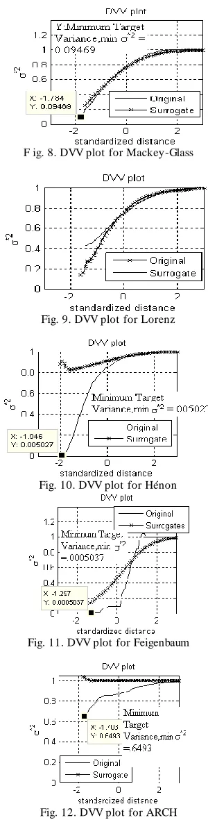
As a result of the standardization of the distance axis rd is replaced by which will have zero mean and unit variance. Then the „DVV plots‟ which are target variance
( ) as a function of the standardized distance are quite
easy to interpret.The minimum target variance,
= , ( )- is a measure of noise present in the
time series. The amount of noise is the prevalence of the stochastic component. The presence of strong deterministic component will lead to small target variance for small spans. At the extreme right, the DVV plots smoothly converges to unity, since for maximum spans, all DVs belong to the same universal set, and the variance of the targets is equal to the variance of the time series.
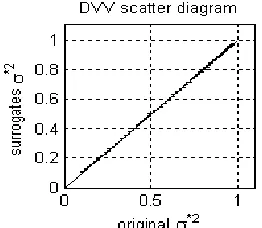
In order to generate surrogate time series, Iterative Amplitude Adjusted Fourier Transform (iAAFT) [9] has been used. With the help of the original and the surrogate time series DVV scatter diagram can be produced, where the horizontal axis corresponds to the DVV plot of the original time series and the vertical to that of the surrogate time series. DVV plots can be interpreted as follows.
If the surrogate time series signal yields DVV plots similar to that of the original time series , the „DVV scatter diagram‟
coincides with the bisector line and original time series is judged to be linear. If the surrogate time series yield DVV plots not similar to that of the original time series , the curve will deviate from the bisector line and original time series is judged to be non-linear. Thus the deviation from the bisector line is an indication of non-linearity, and can be quantified as root mean square error (RMSE) between the s of the original time series and the averaged over the DVV plots of the surrogate time series :
√〈( ( ) ∑
( )
) 〉
(3)
Where ( ) is the target variance at span rd for the i-th surrogate and the average is taken over all span of rd that is valid in all surrogate and DVV plots.
IV. THE ENT ROPY RAT IO(ER) MET HOD
The amount of disorder in time series can be measured by the
Kozachenko-Leonenko(K-L)[10] estimate of the differential entropy
( ) ∑ ( ) (4) where N is the number of samples in the time series , j is the Euclidean distance of the j-th delay vector to its nearest neighbor, and CE(≈ 0.5772) is the Euler constant. For a given embedding dimension, m, and time lag, η , let H(x, m, η) denote the differential entropies estimated for time delay embedded versions of a time series, x. The set of optimal parameters, { mopt, ηopt }, yields a phase space representation which best reflects the dynamics of the underlying signal production system. Therefore, it is expected that this representation has minimal differential entropy (minimal disorder). Thus, optimization of the differential entropy (Eq. 4) for m and η is achieved and the minimum of H(x, m, η) yielding the optimal set of embedding parameters { mopt, ηopt } is obtained. The K-L estimates for the time delay embedded versions of the original time series H(x, m, η), and its surrogates H(xs,i, m, η) are computed using Eq. 4 for increasing m and η (index i refers to the i-th surrogate). To determine the optimal embedding parameters, the ratio
( ) 〈 ( ( )
) 〉
( )
needs to he minimized, where 〈 〉 denotes the average over i. To penalise for higher embedding dimensions, the minimum description length (MDL) method is superimposed, yielding the “entropy ratio” (ER):
( ) ( )( ) (6) where N is the number of delay vectors, which is kept
constant for all values of m and under consideration.
V. CONST RUCT ION OF TIME SERIE
generated which have different degrees of nonlinearity and stochastic nature.
Model 1: Chaotic Mackey-Glass time series which is extensively used in non-linear dynamical system modeling is defined by:
( )
We use x0=0.2 and η =17 to generate the time series.
Model2: Chaotic Lorenz time series which is widely used in continuous dynamical system is considered. This time series is defined by
( )
(8)
where , .The sampling frequency is
taken to be 100 Hz (oversampled) to generate the time series.
Model 3:Hénon map can be written in terms of a single variable with two time delays:
xn+1 = 1 + axn2 + bxn-1 (9)
where a=1.4 and b=0.3. This ensures the Hénon map to be chaotic. This map is widely used in weather forecasting.
Model4: A time is generated by a fully deterministic chaotic
Feigenbaum recursion of the form
Xn=3.57 Xn-1 (1-Xn-1) (10)
where the initial condition is , Xo= 0.7.The stochastic nature is absent here since the model is noise free. Also this model exhibits third order non-linear dependence.
Model 5: A time series is generated by a Autoregressive Conditional Heteroscedastic (ARCH) process of the form
Xn = (1+0.5Xn-12)1/2 n (11)
with the value of the initial observation set to X0 = 0.The sequence { n } are sampled from standard normal distribution. This model is a statistical forecasting model for volatility. It considers the variance of the current error term to be a function of the variances of the previous time periods error terms. It is employed commonly in modeling financial time series that exhibits time varying volatility clustering, i.e. periods of swing followed by periods of relative calm.
Model 6: A time series is generated by a nonlinear moving average process (NLMA) of the form
Xn = n+0.8 n-1 n-2 (12)
where the sequence { n } are sampled from standard normal distribution.
Model 7: A time series is generated by an linear stochastic autoregressive moving average process (ARMA) of the form:
Xn=0.8Xn-1+0.15Xn-2+ n+0.3 n-1 (13)
with X0=1 , X1=0.7 and the sequence { n } is sampled from standard normal distribution. This model contains both moving average and autoregressive terms.
VI. SIMULAT IONS
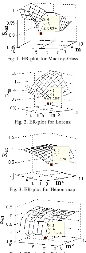
In this section, the Differential entropy based method is used to find out the optimum embedding dimension mopt and the time lag ηopt in order to represent the time series generated by model1 to 7 in phase space. The Entropy-Ratio plot(ER-plot) of the different time series mentioned above is shown in Fig.1 to Fig. 7. These optimum values will be used in DVV method for determining the non-linear and stochastic nature in the time series.
Fig. 1. ER-plot for Mackey-Glass
Fig. 2. ER-plot for Lorenz
Fig. 3. ER-plot for Hénon map
Fig. 5. ER-plot for ARCH
Fig. 6. ER-plot for NLMA
Fig. 7. ER-plot for ARMA
TABLE.I
OP TIMUM VALUES FOR EMBEDDING DIMENSION M AND TIME LAG Τ.
Table I. gives the { mopt, ηopt } for all the time series. Now using these parameters we use DVV method to find out the presence of non-linearity and stochastic nature. The simulation parameters for DVV method are given as: Minimal Size of Set ,λk (rd),N0 =30,Number of surrogates, Ns= 19,Maximal
Span, nd= 3, Number of Reference, DVs = 500, Embedding
Dimension, m and Time Delay, τ are chosen according to
Table.I,
Sample point number
=2000.F ig. 8. DVV plot for Mackey-Glass
Fig. 9. DVV plot for Lorenz
Fig. 10. DVV plot for Hénon
Fig. 11. DVV plot for Feigenbaum
Fig. 12. DVV plot for ARCH T ime Series mopt ηopt
Mackey-Glass 4 6
Lorenz 3 1
Hénon 3 1
Feigenbaum 2 4
ARCH 2 1
NLMA 2 2
Fig. 13. DVV plot for NLMA
Fig. 14. DVV plot for ARMA
Fig. 15. DVV scatter diagram for Mackey-Glass
Fig. 16. DVV scatter diagram for Lorenz
Fig. 17. DVV scatter diagram for Hénon
Fig. 18. DVV scatter diagram for Feigenbaum
Fig. 19. DVV scatter diagram for ARCH
Fig. 20. DVV scatter diagram for NLMA
Fig. 21. DVV scatter diagram for ARMA
VII. DISCUSSION
can conclude that the DVV method has successfully detected the presence of non-linearity as the curves in these figures deviate significantly from the bisector line. This is because the for surrogates are different than that of original time series. For the rest of the three time series namely ARCH, NLMA and ARMA do not have chaotic behavior but non-linearity and stochastic component are present in ARCH and NLMA. DVV method can still successfully indicates the presence of strong stochastic nature in these time series in Fig.12 and Fig.13 by giving a large value of target variance Also, in Fig.19 and Fig.20, the DVV scatter diagram significantly deviates from the bisector line which indicate the non -linear nature in NLMA and ARCH. Finally the time series generated by ARMA process is stochastic but linear. This is clearly shown in Fig.14 where the is 0.1041 which indicates the presence stochastic nature and in Fig .21 linearity is judged as the DVV scatter diagram coincides with the bisector line. So Delay Vector Variance method can successfully determine the presence of nonlinear and stochastic nature in a time series regardless of the fact that whether or not chaos is present. This is possible because DVV method depends on the local predictability of the time series in phase space which can be observed by the target variance of delay vectors (DVs).
REFERENCES
[1] Kaplan, D. ,1994. Exceptional Events as Evidence for Determinism, Physica D, 73,38-48.
[2] Kennel, M.B, Brown, R., & Abarbanel , H.D.I, 1992. Determining Embedding Dimension for Phase Space Reconstruction using a Geometrical Construction, Phys. Rev. A,45, 3403-3411. [3] Schreiber, T & Schmitz, A, 2000. Surrogate T ime Series, Physica D., 142,346-382.
[4] Kaplan, D.,1997. Nonlinearity and Nonstationarity: T he Use of
Surrogate Data in Interpreting Fluctuations in M. Di Rienzo, G. Mancia, G. Parati., A. Pedotti and A. Zanchetti, eds, „Frontiers of Blood Pressure and Heart Rate Analysis‟ IOS press, Amsterdam. [5] Casdagli, M.C. & Weigend, A.S. 1994. Exploring the continuum between deterministic and stochastic modeling, in T ime Series Prediction: Forecasting the Future and Understanding the Past, Reading, MA: Addison-Wesley, 347-367.
[6] Grassberger, P and Procaccia, I., 1983, Measuring the Strangeness of Strange Attractors, Physica D,9, 189-208.
[7] Guatama,T . , Mandic,D.P & Van Hulle,M.M.
4,167-176.
[8] Gautama, T ., Mandic,D.P.,& Van Hulle,M., 2003. A Differential Entropy Based Method for Determining the Optimal Embedding Parameter of a Signal. In Proceedings of ICASSP, Hong-Kong, VI, 29-32.
[9] Kugiumtzis, D. , 1999. T est Your Surrogate before you test your Non-linearity, Phys. Rev. E, 60, 2808-2816.
[10] Beirlant, E.J, Gyorfi, L, Meulen, E.C., 1997. Nonparametric Entropy Estimation: An overview, International J. Mathematical and Statistical Sciences, 6, 17-39.
[11] Barnett, W., Gallant, A., Hinich, M., Jungeilges, J., Kapalan, D. and Jensen, M. 1997 A single Blind Controlled Competition Among T ests for Nonlinearity and Chaos, J. of Econometrics, 77,297-302. [12] Hou ,Shumin., Li ,Yourong and Zhao, Sanxing. Detecting the Nonlinearity in T ime Series from Continuous Dynamic Systems based on Delay Vector Variance Method, J. of Mathematical, Physical and Engineering Sciences.