Modeling & Optimization of Laser Beam Drilling Process Using Genetic Algorithm

Modeling & Optimization of Laser Beam Drilling

Process Using Genetic Algorithm

Dr.G.Harinath Gowd

_,U.Nagaraju

_{, P.Rajesh}

_{, Dr.T.Vishnu Vardhan}

1* _Professor, 1_{Assistant Professor,} 3 _{Associate Professor}

Department of Mechanical Engineering, Madanapalle Institute of Technology & Science, Madanapalle. Andhra Pradesh., INDIA. 2 _{Assistant Professor, Department of Mechanical Engineering, SISTK, PUTTUR, A.P, INDIA}

Email: [email protected]

Abstract— Laser beam machining is one of the modern manufacturing method in this a light can passes to the work material with a high intensity then the material from the stock can be removed and removed molten metal can be ablated by using some gases like Argon, Nitrogen and Oxygen. The execution of any machining operation with best quality is mostly depends on identifying the influenced design variables. The heat affected zone, conical angle of hole, hole taperness, surface roughness..etc. for the desired output responses from the Laser beam drilling operation. In this research, the optimization of hole geometry like as hole diameter at entrance, hole diameter at exit and hole taper are using the Response Surface Methodology (RSM) and Genetic Algorithm (GA). The effects of input variables on the hole diameter at entrance and hole taper are reverse, the problem is expressed as a multi-objective optimization problem.

Index Term-- ND:YAG Laser beam drilling, Empirical modeling, Response Surface methodology, Genetic Algorithm.

1. INTRODUCTION

Laser beam machining is a thermal separation process. In this, there is no physical contact between tool and work piece.

In recent years there is an increasing trend towards miniaturization of various components involving different applications, such as MEMS, electronics, photonics, bio-medical devices [1]

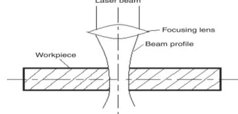
Fig. 1. Schematic diagram of typical laser beam profile.

For getting the best quality of holes using pulsed ND YAG laser machine is mainly depends upon the operating parameters like pulse width, light intensity, gas pressure , type of gas, pulse frequency, beam diameter…etc. using the focusing lenses and reflecting lenses the laser light have high intensity beam. The profile of laser light beam as shown in fig. 1, the hole diameter at exist is differ from hole diameter at entrance in laser drilling operation. It is very difficult to get equal dimensions at both entry and exit of hole [2]. By controlling the process parameters in the pulsed ND YAG laser drilling set up, then it will obtains the dust quality of drilled holes. The jackson was explained the

interaction theory of M2 tool steel in ND YAG pulsed drilling machine [3]. Biswas was researched on the hole circularity and hole taper on TiN-Al2O3 ceramic material [4]. Bandhopadhyay was also investigated on the hole taper angle and hole diameter on the materials of Inconel 718 and Ti-6Al-4V sheets on ND YAG laser [5]. Biswas was also did the research on maximization of hole diameter and minimization of hole taper and the ND YAG micro drilling operation [6]. Ghoreishi was did the analysis of laser percussion drilling operation on the material of mild steel and stainless steel [7]. Yilbas was did the optimization of laser process parameters for hole geometry on Nimonic 75 material [8, 9]. He was also performing the experimentation for optimizing the machine parameters [10]. Kuar was did the research I laser process parameters on heat affected zone (HAZ) and hole taper in pulsed ND YAG laser on the material of zirconium oxide [11]. Low was explained the characterization of spatters on the drilled holes using ND YAG laser [12]. By using the different drilling techniques can optimize the drilled hole circularity [13, 14]. French was explained the analysis of hole taper and circularity in laser percussion drilling [15]. Bandhopadhyay was also explained effects of drilling parameters using Taguchi optimization [16].

Response Surface Methodology:

Response surface methodology (RSM) explores the

relationships between several

explanatory variables

one or more response. The method was introduced by G. E. P.

Box and K. B. Wilson in 1951. The main idea of RSM is to use

a sequence of

designed

said that the usage of this technique is very easy but it can give only approximate solutions but not for the exact solution [17].Response Surface Methodology can give the objective function for the individual responses and analyzing the input

and output variables [18].

The common second-degree polynomial equation for the response is as follows:

…………Eq (1)….

Where Y is the estimated response on a logarithmic scale, x1& x2 are the input variables of the scale, β is the experimental

random error which is normally distributed with mean equals to 0.

2 2

0 1 1 2 2 12 1 2 11 1 22 2

Genetic Algorithm:

Genetic Algorithm(GA) is a search heuristic that mimics the process of natural selection. This heuristic is routinely used to generate useful solutions to optimization and search problems.[19] Genetic algorithms belong to the larger class of evolutionary algorithms (EA), which generate solutions to optimization problems using techniques inspired by natural evolution, such as inheritance, mutation, selection, and crossover.

Fig. 2. Flowchart for GA

2. EXPERIMENTAL WORK

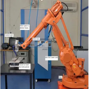
The experiments are directed on high peak power pulsed Nd:YAG Laser drilling machinery with six degrees of freedom robot conveyed through 600 um Luminator fiber., Model Number UW-600A, made by UVWLASERS which is available with Meera Laser Solutions, Ambattor, Chennai, Tamilnadu. The maximum average power produced at laser is 600W.

Fig. 3. Nd:YAG Robotic Laser Drilling equipment

Fig. 4. Work piece after drilling

Fig. 5. Toolmaker’s microscope

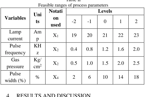
The specifications of the Nd:YAG laser drilling unit is shown in Table.1 The conditions at which the experiments were carried out are detailed in Table 2. Depends upon literature review and DOE, the input variables like Lamp Current (X1), pulse frequency (X2), gas pressure (X3) and pulse width (X4) have major influence on drilled hole diameter and hole taper.

Table I

Specifications of Nd:YAG Laser drilling unit

S.No. Parameter Name Parameter

Data

1 Max. laser power 600W

2 Laser Nd:YAG

3 Wavelength 1064nm

4 Max. single-pulse energy 100J

5 Single-pulse width 0.5ms-30ms

6 Successive pulse width (1

sec.) 200ms/ s

7 Pulse frequency 1-20Hz

responses. These output responses are to be measured by using the Toolmaker’s microscope.

3. DEVELOPMENT OF EMPIRICAL MODELS

MINITAB is one of the optimization software.it can helps to generate the design matrix for 31 different set of conditions. It is used to calculate the regression coefficients for the responses. The Analysis of variance (ANOVA) is used to analyze the relation between factors and responses and then check the adequacy of the model. The P value is should be less than 1, the regression coefficient value should be closer to 1and finally the difference between Squared value and adjusted R-Squared value should be less than 0.05.

Table II

Feasible ranges of process parameters

Variables Uni ts

Notati on used

Levels

-2 -1 0 1 2

Lamp current

Am

p X1 19 20 21 22 23 Pulse

frequency KH

z X2 0.4 0.8 1.2 1.6 2.0 Gas

pressure Kg/

cm2 X2 0.5 1.0 1.5 2.0 2.5

Pulse

width (%) % X4 2 6 10 14 18

4. RESULTS AND DISCUSSION

Table III

Plan of process parameters for experiment, setting as per coding and measured responses

R S.No Input parameters Responses

La mp curr ent

Pulse freque ncy

Gas pres sure

Pu lse wi dth

Diam eter at entra

nce Diam

eter at exit

Hole Taper (radians

)

1 20 0.8 1.0 6 1.015 0.910 0.105 2 22 0.8 1.0 6 1.013 0.896 0.117 3 20 1.6 1.0 6 1.042 0.929 0.113 4 22 1.6 1.0 6 1.030 0.899 0.131 5 20 0.8 2.0 6 1.006 0.899 0.107 6 22 0.8 2.0 6 1.038 0.914 0.123 7 20 1.6 2.0 6 1.010 0.897 0.113 8 22 1.6 2.0 6 1.026 0.901 0.125 9 20 0.8 1.0 14 1.003 0.921 0.082 10 22 0.8 1.0 14 0.962 0.875 0.086 11 20 1.6 1.0 14 1.003 0.925 0.077 12 22 1.6 1.0 14 0.950 0.865 0.085 13 20 0.8 2.0 14 1.010 0.929 0.080 14 22 0.8 2.0 14 1.001 0.924 0.077 15 20 1.6 2.0 14 0.986 0.915 0.070 16 22 1.6 2.0 14 0.968 0.891 0.077 17 19 1.2 1.5 10 1.063 0.966 0.087 18 23 1.2 1.5 10 1.020 0.921 0.098

19 21 0.4 1.5 10 0.984 0.890 0.094 20 21 2.0 1.5 10 0.973 0.881 0.091 21 21 1.2 0.5 10 1.006 0.900 0.106 22 21 1.2 2.5 10 1.016 0.919 0.096 23 21 1.2 1.5 2 1.080 0.932 0.148 24 21 1.2 1.5 18 1.001 0.938 0.063 25 21 1.2 1.5 10 1.021 0.929 0.092 26 21 1.2 1.5 10 1.022 0.929 0.092 27 21 1.2 1.5 10 1.039 0.942 0.097 28 21 1.2 1.5 10 1.038 0.942 0.096 29 21 1.2 1.5 10 1.037 0.939 0.098 30 21 1.2 1.5 10 1.038 0.944 0.094 31 21 1.2 1.5 10 1.034 0.944 0.090

Design Expert 9V, is used to work out the regression coefficients of the suggested model. A general 2nd _order polynomial response surface mathematical model is fitted detailed. The following equations are obtained

𝒚𝒅𝒊𝒂𝒎𝒆𝒕𝒆𝒓𝒂𝒕𝒆𝒙𝒊𝒕= 𝟎. 𝟗𝟒 − 𝟎. 𝟎𝟐𝟏𝒙𝟏− 𝟎. 𝟎𝟎𝟓𝟑𝟑𝟑𝒙𝟐+ 𝟎. 𝟎𝟎𝟕𝟑𝟑𝟑𝒙𝟑+

𝟎. 𝟎𝟎𝟏𝟎𝟎𝒙𝟒− 𝟎. 𝟎𝟏𝟓𝒙𝟏𝒙𝟐+ 𝟎. 𝟎𝟑𝟓𝒙𝟏𝒙𝟑− 𝟎. 𝟎𝟐𝟕𝒙𝟏𝒙𝟒− 𝟎. 𝟎𝟏𝟗𝒙𝟐𝒙𝟑−

𝟎. 𝟎𝟏𝟓𝒙_𝟐𝒙_𝟒+ 𝟎. 𝟎𝟐𝟒𝒙_𝟑𝒙_𝟒− 𝟎. 𝟎𝟎𝟑𝟒𝟐𝟗𝒙_𝟏𝟐_{− 𝟎. 𝟎𝟔𝟏𝒙} 𝟐

𝟐_{− 𝟎. 𝟎𝟑𝟕𝒙} 𝟑 𝟐₋

𝟎. 𝟎𝟏𝟐𝒙_𝟒𝟐

Eq……(3)

𝒚𝒉𝒐𝒍𝒆𝒕𝒂𝒑𝒆𝒓=𝟎. 𝟗𝟒 + 𝟎. 𝟎𝟎𝟖𝟎𝟎𝒙𝟏+ 𝟎. 𝟎𝟎𝟎𝟔𝟔𝟔𝟕𝒙𝟐− 𝟎. 𝟎𝟎𝟑𝟔𝟔𝟕𝒙𝟑−

𝟎. 𝟎𝟑𝟗𝒙𝟒+ 𝟎. 𝟎𝟎𝟒𝟎𝒙𝟏𝒙𝟐− 𝟎. 𝟎𝟎𝟐𝟓𝟎𝒙𝟏𝒙𝟑− 𝟎. 𝟎𝟏𝟏𝒙𝟏𝒙𝟒−

𝟎. 𝟎𝟎𝟒𝟓𝟎𝒙𝟐𝒙𝟑− 𝟎. 𝟎𝟏𝟐𝒙𝟐𝒙𝟒− 𝟎. 𝟎𝟎𝟕𝟎𝒙𝟑𝒙𝟒− 𝟎. 𝟎𝟎𝟏𝟓𝟔𝟎𝒙𝟏𝟐−

𝟎. 𝟎𝟎𝟏𝟓𝟔𝟎𝒙𝟐𝟐+ 𝟎. 𝟎𝟎𝟔𝟗𝟒𝟎𝒙𝟑𝟐+ 𝟎. 𝟎𝟏𝟏𝒙𝟒𝟐

Table IV

ANOVA [Partial sum of squares] for Hole diameter at exit

Source Sum of

Squares d. f.

Mean

Square F-Value Prob> F

Model 0.015 14 1.075E-003 14.44 0.0001*

x1 2.604E-003 1 2.604E-003 34.99 0.0001* x2 1.707E-004 1 1.707E-004 2.29 0.1495 x3 3.227E-004 1 3.227E-004 4.33 0.0538

x4 6.00E-006 1 6.00E-006 0.081 0.7801

x1x2 2.250E-004 1 2.250E-004 3.02 0.1013 x1x3 1.225E-003 1 1.225E-003 16.46 0.0009 x1x4 7.562E-004 1 7.562E-004 10.16 0.0057 x2x3 3.802E-004 1 3.802E-004 5.11 0.0381 x2x4 2.250E-004 1 2.250E-004 3.02 0.1013 x3x4 5.760E-004 1 5.760E-004 7.74 0.0133 x12 2.101E-005 1 2.101E-005 0.28 0.6025 x22 6.744E-003 1 6.744E-003 90.60 0.0001* x32 2.504E-003 1 2.504E-003 33.64 0.0001* x42 2.543E-004 1 2.543E-004 3.42 0.0831

Residual 1.191E-003 16 7.444E-005

Pure Error 2.657E-004 6 4.429E-005

Cor Total 0.016 30

Std. Dev. 8.628E-003 R2 0.9266

Mean 0.92 Adj. R2 0.8625

Table V

ANOVA [Partial sum of squares] for Hole taper

Source Sum of Squares

d. f. Mean Square

F-Value Prob> F

Model 0.010 14 7.383E-004 74.32 0.0001*

x1 3.840E-004 1 3.840E-004 38.66 0.0001*

x2 2.667E-006 1 2.667E-006 0.27 0.6115

x3 8.067E-005 1 8.067E-005 8.12 0.0116

x4 9.204E-003 1 9.204E-003 926.55 0.0001*

x1x2 1.600E-005 1 1.6E-005 1.61 0.2225

x1x3 6.250E-006 1 6.250E-006 0.63 0.4393

x1x4 1.103E-004 1 1.103E-004 11.10 0.0042

x2x3 2.025E-005 1 2.025E-005 2.04 0.1726

x2x4 1.323E-004 1 1.323E-004 13.31 0.0022

x3x4 4.9E-005 1 4.9E-005 4.93 0.0411

x12 4.347E-006 1 4.347E-006 0.44 0.5177

x22 4.347E-006 1 4.347E-006 0.44 0.5177

x32 8.609E-005 1 8.609E-005 8.67 0.0095

x42 2.339E-004 1 2.339E-004 23.55 0.0002

Residual 1.589E-004 16 9.934E-006 Pure Error 5.286E-005 6 8.81E-006

Cor Total 0.010 30

Std. Dev. 3.152E-003 R2 _0.9849

Mean 0.097 Adj. R2 _0.9716

Fig. 6. Normal probability of residuals for hole taper

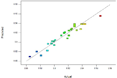
Fig. 7. Predictive Vs Actual values for hole taper

Fig. 8. Normal probability of residuals for hole diameter at exit

Fig. 9. Predictive Vs Actual values for hole diameter at exit

In this research work, the goal is to maximize the hole diameter at exit and minimize the hole taper, which forms the multi objective optimization problem. Hole diameter at exit and hole taper denotes in the Equation 3 and 4, correspondingly. The difficulties of the models were minimized by using the back elimination process. After eliminating the minor relations, the final equations are as shown below:

𝒚𝒅𝒊𝒂𝒎𝒆𝒕𝒆𝒓𝒂𝒕𝒆𝒙𝒊𝒕= 𝟎. 𝟗𝟒 − 𝟎. 𝟎𝟐𝟏𝒙𝟏− 𝟎. 𝟎𝟎𝟓𝟑𝟑𝟑𝒙𝟐

+ 𝟎. 𝟎𝟎𝟕𝟑𝟑𝟑𝒙𝟑+ 𝟎. 𝟎𝟎𝟏𝟎𝟎𝒙𝟒

𝒚𝒉𝒐𝒍𝒆𝒕𝒂𝒑𝒆𝒓= 𝟎. 𝟗𝟒 + 𝟎. 𝟎𝟎𝟖𝟎𝟎𝒙𝟏+ 𝟎. 𝟎𝟎𝟎𝟔𝟔𝟔𝟕𝒙𝟐

− 𝟎. 𝟎𝟎𝟑𝟔𝟔𝟕𝒙𝟑− 𝟎. 𝟎𝟑𝟗𝒙𝟒

+ 𝟎. 𝟎𝟎𝟒𝟎𝒙𝟏𝒙𝟐− 𝟎. 𝟎𝟎𝟐𝟓𝟎𝒙𝟏𝒙𝟑 − 𝟎. 𝟎𝟏𝟏𝒙𝟏𝒙𝟒− 𝟎. 𝟎𝟎𝟒𝟓𝟎𝒙𝟐𝒙𝟑 − 𝟎. 𝟎𝟏𝟐𝒙𝟐𝒙𝟒− 𝟎. 𝟎𝟎𝟕𝟎𝒙𝟑𝒙𝟒 − 𝟎. 𝟎𝟎𝟏𝟓𝟔𝟎𝒙𝟏𝟐− 𝟎. 𝟎𝟎𝟏𝟓𝟔𝟎𝒙𝟐𝟐 + 𝟎. 𝟎𝟎𝟔𝟗𝟒𝟎𝒙𝟑𝟐+ 𝟎. 𝟎𝟏𝟏𝒙𝟒𝟐 In the above equations, x1, x2, x3, and x4 represent the logarithmic transformations of Lamp current, pulse frequency, Gas pressure, and pulse width respectively, and they are given below:

Table VI

Feasible bounds of control variables

Variable Lower limit Upper limit

Lamp Current (X1) 19 23

Pulse frequency(X2) 0.4 2

Gas pressure(X3) 0.5 2.5

Pulse width(X4) 2 19

X1=

ln(𝑋1)−ln⁡(20) ⁡ln(22)−ln⁡(20) , X2 =

ln(𝑋2)−ln⁡(1.6)

⁡ln(1.8)−ln⁡(1.6) X3 =

ln(𝑋3)−ln⁡(1.5)

⁡ln(2.0)−ln⁡(1.5) X4 =

ln(𝑋4)−ln⁡(15)

⁡ln(17)−ln⁡(15)……Eq (5)

The above relations were obtained from the following transformation equation:

X =

ln(𝑋𝑛)−ln⁡(𝑋𝑛𝑜)

⁡ln(1.8𝑋𝑛1)−ln⁡(𝑋𝑛𝑜) ………..Eq (6)

Where X is the coded value X n is the natural value

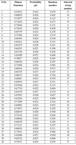
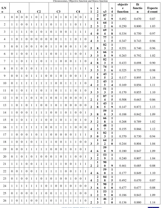
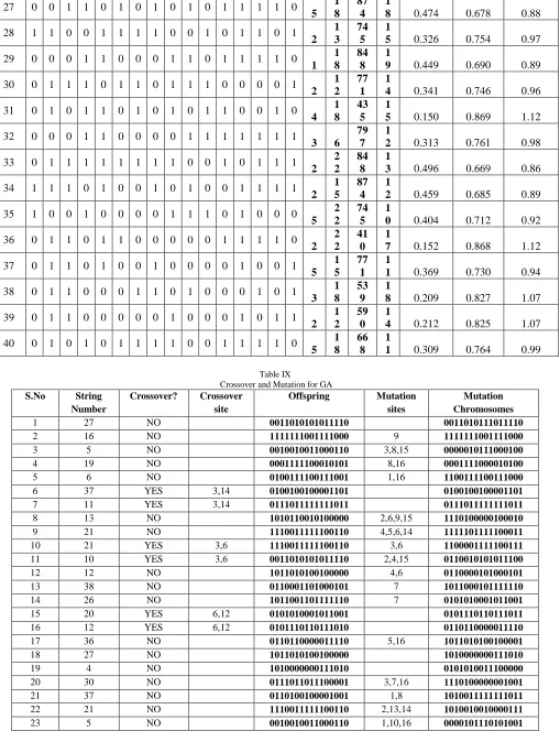
X n1 is the natural value of the factor at lower limit X n0 is the natural value of factor at upper limit; In the table.6 the upper and lower limit of the factors are to be furnished. In the tables VII, VIII, and IX are indicate the step by step procedure for the genetic algorithm optimization.

Table VIII Selection of GA

S.No Fitness Function

Probability (pi)

Random number

Selected string number

1 0.67032 0.022 0.678 27

2 0.80029 0.026 0.403 16

3 0.74977 0.024 0.125 5

4 0.74263 0.024 0.473 19

5 0.74044 0.024 0.131 6

6 0.79183 0.026 0.920 37

7 0.69779 0.023 0.278 11

8 0.75496 0.024 0.319 13

9 0.89494 0.029 0.540 21

10 0.85561 0.028 0.535 21

11 0.85475 0.028 0.251 10

12 0.66291 0.021 0.298 12

13 0.87198 0.028 0.936 38

14 0.84200 0.027 0.668 26

15 0.78877 0.025 0.505 20

16 0.86556 0.028 0.297 12

17 0.72986 0.024 0.902 36

18 0.80416 0.026 0.673 27

19 0.84745 0.027 0.107 4

20 0.80675 0.026 0.704 30

21 0.68467 0.022 0.970 37

22 0.84934 0.027 0.531 21

23 0.67046 0.022 0.115 5

24 0.67720 0.022 0.004 1

25 0.84339 0.027 0.334 14

26 0.87992 0.028 0.827 33

27 0.67826 0.022 0.090 4

28 0.75389 0.024 0.516 20

29 0.69003 0.022 0.852 34

30 0.74597 0.024 0.302 12

31 0.86919 0.028 0.940 38

32 0.76145 0.025 0.846 34

33 0.66856 0.022 0.202 8

34 0.68538 0.022 0.269 11

35 0.71221 0.023 0.197 8

36 0.86834 0.028 0.311 13

37 0.73021 0.024 0.896 36

38 0.82688 0.027 0.950 38

39 0.82532 0.027 0.068 3

Table VII

Chromosomes, Objective function and fitness function

S.N

o C1 C2 C3 C4

x 1

x 2 x3

x 4 objectiv e function fit functio n Expecte d count

1 0 0 0 0 1 0 1 1 1 0 1 0 1 0 0 1

1 2 0 87 4 1

9 0.492 0.670 0.87

2 1 1 0 0 1 1 1 1 0 1 1 1 1 0 1 1

2 1 3 64 2 1

6 0.250 0.800 1.03

3 1 1 1 1 0 1 0 1 0 1 0 0 1 1 1 1

4 2 0 69 4 1

8 0.334 0.750 0.97

4 1 0 1 0 0 0 0 0 0 0 1 1 1 0 1 0

4 1 3 77 1 1

5 0.347 0.743 0.96

5 0 0 1 0 0 1 0 0 1 1 0 0 0 1 1 0

5 8 82

3 1

2 0.351 0.740 0.96

6 0 1 0 0 1 1 1 1 0 0 1 1 1 0 0 1

3 1 3 66 8 1

9 0.263 0.792 1.02

7 1 1 0 1 1 1 0 1 1 1 0 0 0 1 1 0

4 1 8 82 3 1

5 0.433 0.698 0.90

8 0 1 0 1 0 1 1 1 1 1 1 1 1 1 1 1

3 1 3 74 5 1

6 0.325 0.755 0.98

9 0 0 1 0 1 1 1 0 0 1 0 1 0 0 1 1

5 1 0 43 5 1

2 0.117 0.895 1.16

10 0 1 1 1 1 1 1 1 1 0 0 1 1 1 1 0

4 2 2 43 5 1

4 0.169 0.856 1.11

11 0 1 0 1 1 1 0 1 1 0 1 1 1 0 1 0

3 1 3 51 3 1

5 0.170 0.855 1.10

12 1 0 1 1 0 1 0 1 0 0 1 0 0 0 0 1

2 2 1 87 4 1

5 0.508 0.663 0.86

13 1 0 1 0 1 1 0 0 1 0 1 0 0 0 0 0

2 1 8 43 5 1

9 0.147 0.872 1.13

14 1 0 0 0 1 1 1 1 0 0 1 0 1 0 0 1

3 8 59

0 1

3 0.188 0.842 1.09

15 0 1 0 1 1 1 1 0 0 1 0 1 1 0 1 0

3 1 2 66 8 1

1 0.268 0.789 1.02

16 1 1 1 1 1 1 1 0 0 1 1 1 1 0 0 0

4 1 3 48 7 1

5 0.155 0.866 1.12

17 1 0 0 0 1 0 1 1 0 0 0 0 0 1 1 1

5 1 0 82 3 1

1 0.370 0.730 0.94

18 1 0 0 1 0 1 1 1 1 0 0 1 1 1 0 0

3 1 3 64 2 2

0 0.244 0.804 1.04

19 0 0 0 1 1 1 1 1 0 0 0 1 0 1 0 1

4 6 59

0 9 0.180 0.847 1.09

20 0 1 0 1 0 1 0 0 0 1 0 1 1 0 0 1

3 2 2 53 9 1

1 0.240 0.807 1.04

21 1 1 1 0 0 1 1 1 1 1 1 0 0 1 1 1

2 1 2

90

0 9 0.461 0.685 0.88

22 0 0 1 0 0 1 1 1 1 1 1 0 0 1 1 1

4 6 59

0 1

1 0.177 0.849 1.10

23 0 1 0 0 1 1 0 1 0 1 0 0 1 0 0 1

4 2 2 84 8 1

5 0.492 0.670 0.87

24 1 1 1 1 1 1 1 0 1 0 0 1 0 1 0 0

3 1 6 90 0 2

0 0.477 0.677 0.88

25 0 1 0 0 0 1 1 0 0 1 1 1 1 1 0 0

1 1 2 53 9 1

0 0.186 0.843 1.09

26 1 0 1 1 0 0 1 1 0 1 1 1 1 1 1 0

2 1 3 46 1 2

27 0 0 1 1 0 1 0 1 0 1 0 1 1 1 1 0 5

1 8

87 4

1

8 0.474 0.678 0.88

28 1 1 0 0 1 1 1 1 0 0 1 0 1 1 0 1

2 1 3

74 5

1

5 0.326 0.754 0.97

29 0 0 0 1 1 0 0 0 1 1 0 1 1 1 1 0

1 1 8

84 8

1

9 0.449 0.690 0.89

30 0 1 1 1 0 1 1 0 1 1 1 0 0 0 0 1

2 1 2

77 1

1

4 0.341 0.746 0.96

31 0 1 0 1 1 0 1 0 1 0 1 1 0 0 1 0

4 1 8

43 5

1

5 0.150 0.869 1.12

32 0 0 0 1 1 0 0 0 0 1 1 1 1 1 1 1

3 6 79

7 1

2 0.313 0.761 0.98

33 0 1 1 1 1 1 1 1 1 0 0 1 0 1 1 1

2 2 2

84 8

1

3 0.496 0.669 0.86

34 1 1 1 0 1 0 0 1 0 1 0 0 1 1 1 1

2 1 5

87 4

1

2 0.459 0.685 0.89

35 1 0 0 1 0 0 0 0 1 1 1 0 1 0 0 0

5 2 2

74 5

1

0 0.404 0.712 0.92

36 0 1 1 0 1 1 0 0 0 0 0 1 1 1 1 0

2 2 2

41 0

1

7 0.152 0.868 1.12

37 0 1 1 0 1 0 0 1 0 0 0 0 1 0 0 1

5 1 5

77 1

1

1 0.369 0.730 0.94

38 0 1 1 0 0 0 1 1 0 1 0 0 0 1 0 1

3 1 8

53 9

1

8 0.209 0.827 1.07

39 0 1 1 0 0 0 0 0 1 0 0 0 1 0 1 1

2 1 2

59 0

1

4 0.212 0.825 1.07

40 0 1 0 1 0 1 1 1 1 0 0 1 1 1 1 0

5 1 8

66 8

1

1 0.309 0.764 0.99

Table IX

Crossover and Mutation for GA

S.No String Number

Crossover? Crossover site

Offspring Mutation sites

Mutation Chromosomes

1 27 NO 0011010101011110 0011010111011110

2 16 NO 1111111001111000 9 1111111001111000

3 5 NO 0010010011000110 3,8,15 0000010111000100

4 19 NO 0001111100010101 8,16 0001111000010100

5 6 NO 0100111100111001 1,16 1100111100111000

6 37 YES 3,14 0100100100001101 0100100100001101

7 11 YES 3,14 0111011111111011 0111011111111011

8 13 NO 1010110010100000 2,6,9,15 1110100000100010

9 21 NO 1110011111100110 4,5,6,14 1111101111100011

10 21 YES 3,6 1110011111100110 3,6 1100001111100111

11 10 YES 3,6 0011010101011110 2,4,15 0110010101011100

12 12 NO 1011010100100000 4,6 0110000101000101

13 38 NO 0110001101000101 7 1011000101111110

14 26 NO 1011001101111110 7 0101010001011001

15 20 YES 6,12 0101010001011001 0101110110111011

16 12 YES 6,12 0101110110111010 0110110000011110

17 36 NO 0110110000011110 5,16 1011010100100001

18 27 NO 1011010100100000 1010000000111010

19 4 NO 1010000000111010 0101010011100000

20 30 NO 0111011011100001 3,7,16 1110100000001001

21 37 NO 0110100100001001 1,8 1010011111111011

24 1 NO 0000101110101001 1100011100101001

25 14 YES 2,5 1100011100101000 1110010010100000

26 33 YES 2,5 1110010010100000 1010000000111010

27 4 NO 1010000000111010 010100001001001

28 20 YES 6,12 0101000001001001 1110110101011111

29 34 YES 6,12 1110110101011110 0101011110111111

30 12 YES 10,11 0101011110111111 0011010101111110

31 38 YES 10,11 0011010101111110 0101010001011001

32 34 NO 0101010001011001 0100011111111111

33 8 NO 0101011111111111 4 0101110110110010

34 11 NO 0101110110111010 13 0111110100101000

35 8 NO 0101110110111010 3,9,12,15 0111111110010011

36 13 NO 0111111110010111 14 1010010010000111

37 36 NO 0110110000011110 3,13 0100110000010110

38 38 NO 0110001101000101 9 0110001111000101

39 3 NO 1111010101001110 1,13,16 0111010101000110

40 27 NO 0111111110101110 0111111110101110

CONCLUSIONS

In the present study, Design based experiments and analysis have been carried out in order to optimize the hole taper considering the effects of lamp current, pulse frequency, gas pressure and pulse width of AISI 304L using ND:YAG robot assisted Laser beam drilling setup. Later A constrained optimization problem is then formulated to minimize the hole taper subject to the hole diameter at entrance and exit as constraints. A binary coded Genetic algorithm was used to solve the above said problem. GA based optimality analysis achieve better fitness function values as compared to those derived by the past researchers. Through GA, minimum hole taper obtained is 0.062 rad. The result suggests that average to low values of nitrogen pressure and pulse width combined with average to high values of pulse frequency and lamp current gives optimal results for minimum hole taper. In summary, the proposed work enables the manufacturing engineers to select the optimal values depending on the production requirements and as a consequence, automation of the process could be done based on the optimal values.

REFERENCES

[1] Steen WM, Mazumder J. Laser material processing. 4th ed.New York: Springer; 2010.

[2] Chen TC, Robert B, Darling RB. Parametric studies on pulsednear ultraviolet frequency tripled Nd:YAG lasermicromachining of sapphire and silicon. J Mater ProcessTechnol 2005;169:214–8.

[3] MJ, O’Neill W. Laser micro-drilling of tool steel usingNd:YAG lasers. J Mater Process Technol 2003;142:517–25.

[4] Biswas R, Kuar AS, Biswas SK, Mitra S. Artificial neuralnetwork modeling of Nd:YAG laser microdrilling on titaniumnitride–alumina composite. Proc Inst Mech Eng B: J EngManuf 2010;224(B3):473–82

[5] Bandhopadhayay S, Sarin Sundar JK, Sunderajan G, Joshi SV.Geometrical features and metallurgical characteristics ofNd:YAG laser drilled holes in thick IN718 and Ti-6Al-4Vsheets. J Mater Process Technol 2002;127:83–95

[6] Biswas R, Kuar AS, Biswas SK, Mitra S. Effects of processparameters on hole circularity and taper in pulsed Nd:YAGlaser micro-drilling of TiN–Al2O3composites. Mater ManufProcess 2010;25(6):503–14

[7] Ghoreishi M, Low DKY, Li L. Comparative statistical analysisof hole taper and circularity in laser percussion drilling. Int JMach Tools Manuf 2002;42:985–95

[8] Yilbas BS, Yilbas Z. Parameters affecting hole geometry inlaser drilling of Nimonic 75. SPIE 1987;744:87–91

[9] Yilbas BS. Investigation into drilling speed during laserdrilling of metals. J Opt Laser Technol 1988;20(1):29–32.

[10] Yilbas BS. Parametric study to improve laser hole drillingprocess. J Mater Process Technol 1997;70:264–73. [11] Kuar AS, Doloi B, Bhattacharyya B. Modelling and analysis

ofpulsed Nd:YAG laser machining characteristics duringmicro-drilling of zirconia (ZrO2). Int J Mach Tools Manuf2006;46:1301–10.

[12] Low DKY, Li L, Corfe AG. Characteristics of spatter formationunder the effects of different laser parameters during laserdrilling. J Mater Process Technol 2001;118:179–86. [13] Low DKY, Li L, Byrd PJ. Taper formation and control

duringlaser drilling in Nimonic 263 alloy. In: Proceedings of 33rdInternational MATADOR Conference. UMIST; 2000. p. 461–6.

[14] Low DKY, Li L, Corfe AG, Byrd PJ. Taper control during laserpercussion drilling of nimonic alloy using sequential pulsedelivery pattern control (SPDPC). In: Proceedings of ICALEO.1999. p. 11–20.

[15] French PW, Hand DP, Peters C, Shannon GJ, Byrd P, Watkins K,Steen WM. Investigation of Nd:YAG laser percussion drillingprocess using factorial experimental design. In: Proceedingsof ICALEO. 1999. p. 51–60.

[16] Bandhopadhayay S, Gokhale H, Sarin Sundar JK, SundarajanG, Joshi SV. A statistical approach to determine processparameters impact in Nd:YAG laser drilling of IN718 andTi-6Al-4V sheets. Opt Lasers Eng 2005;43:163–82.

[17] Box GEP, Wilson KB (1951) Experimental attainment of optimum conditions. J R Stat Soc [Ser A] 13:1–45

[19] Mitchell, Melanie (1996). An Introduction to Genetic Algorithms. Cambridge, MA: MIT Press. .

[20] Montgomery DC (2001) Design and analysis of experiments Wiley, Hoboken

[21] Minitab (2003) Software Version 14, User’s Guide, Technical

Manual. Minitab, State College.