ORIGINAL PAPER
Drivers of changes in Spanish accessibility for the 1960
–
2010
period
Ana Condeço-Melhorado1,2 &José Luis Zofío3&Panayotis Christidis2
Received: 4 November 2015 / Accepted: 10 March 2017 / Published online: 1 April 2017 #The Author(s) 2017. This article is published with open access at SpringerLink.com
Abstract
PurposeThe accessibility of a certain place can evolve either as the direct result of transport changes or as a consequence of the spatial redistribution of economic activities. These two factors are often indistinguishable—especially at regional level—since improved infrastructure stimulates relocation of activities. Moreover, infrastructure investment choices tend to follow population and economic activity patterns, distorting the cause and effect relationship between infrastructure and accessibility even further. The methodology and results pre-sented here decompose the impact of both factors in terms of accessibility using Spanish data between 1960 and 2010. During this period, Spain experienced profound changes in transport infrastructure and economic activity.
Methods We use the potential accessibility indicator and re-sort to index number theory to disentangle the contribution of transport infrastructure from that of land-use changes. Detailed historical data on road infrastructure and population
is used to represent the transport and land-use components of accessibility.
Results Our results show that changes in transport infrastruc-ture had a relevant impact on accessibility, as expected, but changes in the spatial distribution of population had an even greater effect. This outcome may be used as an argument for sustainable accessibility, a concept that advocates integration of transport and land use planning.
Keywords Historical accessibility . Transport infrastructure assessment . Population change . Productivity index
1 Introduction
There is a growing trend in the literature on transport planning that advocates a change of paradigm from mobility to acces-sibility planning ([1–5]). Mobility-based measures that have dominated many transport policies include delay per capita, monetary cost of congestion, and highway level of service. Behind the mobility approach, travel speed is considered to be a fundamental key to transport policy success. However, many of those arguing for a paradigm change recall that mo-bility is rarely an end in itself, but rather a means to increase accessibility [6]. People move towards opportunities and thus the ultimate objective of transport policies should be maximising accessibility instead of speed.
The accessibility concept may be defined as ease of access to markets and it is usually related with lower transport costs, higher levels of competitiveness and better quality of life. This concept has the advantage of simultaneously showing the quality of transport systems (infrastructure) and the location of activities (land-use). An improvement in transport infra-structure, such as constructing a new highway, will reduce travel time and increase accessibility. While, (re)location of
Disclaimer: The views expressed are purely those of the authors and may not in any circumstances be regarded as stating an official position from the European Commission
This article is part of the Topical Collection on Accessibility and Policy Making
* Ana Condeço-Melhorado
1
Universidad Complutense de Madrid, C/ Profesor Arangüren s/n, 28040 Madrid, Spain
2
European, Commission, Joint Research Centre, C/Inca Garcilaso, 3, E-41092 Seville, Spain
3 Universidad Autónoma de Madrid, C/Francisco Tomás y Valiente, 5.,
economic activities, will change job opportunities for resi-dents in the surrounding areas.
However, in the long run, the effects of transport infrastruc-ture and land uses on accessibility may merge. New economic geography literature suggests that the relationship between transport investments and changes in activity patterns does not always favour economic cohesion but may result in core-periphery distributions [7]. Decreasing returns of trans-port investments have been measured by several authors ([8, 9]). This is also true for accessibility, since accessibility impacts decrease with network density.
In addition, increased transport capacity may induce spatial dispersion of economic activities, resulting in longer and cost-lier trips. Spence and Linneker [10] studied the relationship between regional employment and accessibility changes due to new motorways. Their results showed that employment growth was higher in areas with low accessibility, suggesting a decentralization process of economic activities.
Conversely, the agglomeration of economic activities usu-ally entails higher congestion levels which negatively affect accessibility, through increasing transport costs. Nonetheless, most of the more accessible regions also have the highest congestion levels.
It is clear that accessibility is a function of transport infra-structure and the location of economic activities, but which of the two conjoint effects will have a higher impact on accessi-bility changes? And how does the weight of these two factors evolve over time?
The present study attempts to answer these questions by proposing a new methodology and analysing accessibility change in Spain at the NUTS-3 level, over a 50 year period between 1960 and 2010. During this period a significant trans-formation of transport infrastructure and economic activity took place. We do so by applying index number theory, which allows us to aggregate (i.e. summarize into a single scalar) the bilateral relation between a given location (origin) and its sur-rounding destinations (e.g. commercial partners), considering infrastructure as the main input yielding accessibility to eco-nomic opportunities. Infrastructure, in the form of travel time, is considered as the input producing accessibility to markets as output, resulting in a productivity index that is defined as the ratio of potential economic opportunities to infrastructure. Furthermore, resorting to the product rule of index numbers, we can consistently decompose accessibility change across locations and over time, enabling us to disentangle the contri-bution of transport infrastructure from the land-use dimension. The next section reviews previous studies devoted to the effects of transport infrastructure and land-use on accessibility change, and discusses the advantages of index number theory when pursuing this objective. The following sections present the data and statistical sources used for this analysis (section3) and the methodology employed to measure accessibility change and decompose it into suitable infrastructure and land
use components (section4). Section5reports the results for the Spanish case, while section6draws the main conclusions.
2 Accessibility dimensions and their decomposition
In the literature, there are several indicators that can be used to measure accessibility, each one capable of showing one or several of the following dimensions [11]:
& Land-use: represents the amount and spatial distribution of opportunities at destinations. Opportunities can be mea-sured as population, jobs or other socio-economic variables that may characterize the economic importance of places;
& Transport: describes the transport system as a facilitator of movements (both passenger and freight flows) between an origin and destination. This is commonly represented by time or cost variables reflecting the quality of the transport system;
& Time: captures the potential to access a certain location, depending on factors such as time budgets or opening hours of available opportunities;
& Individual: accessibility is a characteristic of individuals and varies according to their socio-economic status (i.e. income, age, education level).
Given the aggregate national scope of our analysis we will focus on the contribution of the first two dimensions, while time and individual aspects of accessibility are better looked at using micro-level approaches.
Only a few studies evaluate both the contribution of trans-port and land use dimensions to accessibility levels. Spence and Linneker provide one of the first attempts to analyse the evolution of motorways and changing levels of employment on accessibility in Great Britain [10]. Using a standard market potential indicator, these authors show a positive effect of motorways on accessibility levels and some negative impacts due to decentralization of employment, mainly in London and the cities surrounding it.
For the Netherlands, Geurs and Ritsema van Eck, study the effect of transport infrastructure (further subdivided into changes in infrastructure and changes in congestion) and the land use component (measured as the number of jobs), as well as impacts from the interaction of both components [18]. Authors found a higher overall accessibility increase due to changes in employment levels, a lower positive contribution of infrastructure expansion and a negative contribution of the congestion and interaction components.
At a metropolitan level, an interesting study decomposes accessibility into speed and proximity effects for several pairs of US metropolitan regions, [6]. In overall terms, authors show a positive relationship between area density and
accessibility, given the greater weight of origin-destination proximity. They have also shown that increasing urban densi-ty improves the number of jobs and services 10 times more than a proportional change in travel speed.
Some studies look at longer periods of time, individualiz-ing the contribution of population and/or transport infrastruc-ture change to accessibility ([21,22]). However, depending on the study’s objective, the separate contribution from accessi-bility components is omitted.
Despite attempts in the literature to draw conclusions on the contribution of different accessibility dimensions to the overall variation of accessibility levels, the use of different methodologies and case studies make them difficult to com-pare. In this study we use index number theory to define and decompose accessibility variation into mutually exclusive transport infrastructure and land-use components ([23,24]). Specifically, we define a productivity index that relates the infrastructure component to land-use, where the latter can be consistently used to recover the former by means of the prod-uct rule (and vice versa).
One of the main advantages of analysing accessibility levels and its determinants using index number theory is that
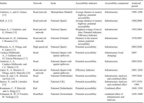
Table 1 Selected accessibility studies looking at different accessibility components
Studies Network Scale Accessibility indicator Accessibility component Analysed
period
Gutiérrez, J., and G. Gómez [12]
Road network Metropolitan (Madrid) Average distance to nearest
highway; potential accessibility
Infrastructure 1990–1996
Holl, A. [13] Road network National (Spain) Average distance to nearest
highway; potential accessibility
Infrastructure 1980/2000
López, E., J. Gutiérrez, and G. Gómez [14]
Road and rail network
National (Spain) Weighted average of travel
time; Potential indicator; Efficiency Indicator
Infrastructure 1992/2004
Kotavaara O., H. Antikainen, J. Rusanen [16]
Road and rail network
National (Finland) Distance to the nearest
station; potential accessibility
Infrastructure 1970/2007
Monzón, A., E. Ortega, and E. López [15]
High speed rail National (Spain) Potential accessibility Infrastructure 2005/2020
Condeço-Melhorado, A., J. Gutiérrez and J.C.García-Palomares [17]
Road National (Spain) with
spatial spillovers
Potential accessibility Infrastructure (road
charging)
2005
Gutiérrez, J., A.
Condeço-Melhorado, and J. C. Martín [19]
Road National (Spain) with
spatial spillovers
Potential accessibility Infrastructure 2005/2020
López, E., A. Monzón, E. Ortega, and S. Mancebo [20]
Road and rail network
National (Spain) with spatial spillovers
Efficiency Indicator Infrastructure 2005–2020
Geurs, K. and, J. R., Ritsema van Eck [18]
Road National (Netherlands) Potential accessibility Infrastructure, land-use
and combined effect
1995/2020
Spence, N., and B. Linneker [10]
Road National (UK) Potential accessibility Infrastructure, land-use
and combined effect
1971/1976/ 1989 Koopmans, C., P. Rietveld,
and A. Huijg [21]
Rail National (Netherlands) Potential accessibility Combined effect 1840–1930
Axhausen, K. W., P. Froelich, M. Tschopp [22]
Road/Rail National (Switzerland) Potential accessibility combined effect of
Infrastructure and land-use
this type of approach allows comparability with other studies that may use the same methodology in other places and times. In addition, we improve the methodology to accurately mea-sure the change in accessibility and provide a consistent de-composition of these changes, which allows us to draw con-clusions on the precise effects of transport infrastructure and population determinants.
Zofío, J. L. et al. have applied this methodology to study the drivers of generalized transport cost evolution, basically economic costs and infrastructure [25] although as far as we know, this is the first time basic index number theory has been used to estimate the relative contribution of different accessi-bility components, namely, transport infrastructure and land use dimensions.
Another contribution from this study is the use of historical data to measure the contribution from these two components to accessibility change, covering a long time period (50 years) and providing outcomes for every decade within this period.
3 Data
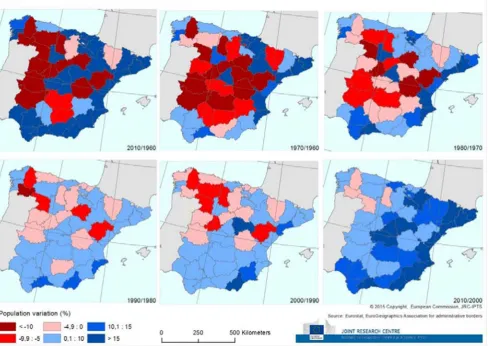
To calculate accessibility changes in Spain, we use Eurostat population data for the 47 Spanish NUTS 3 regions (islands are excluded), representing 1960, 1970, 1980, 1990, 2000 and 2010. NUTS 3 regions are represented by their centroids (the regional central point) for distance matrix calculations, while NUTS 3 boundaries are used to represent accessibility chang-es in maps. NUTS 3 regions seemed the most appropriate level of analysis given the relatively low spatial detail of the road network (presented below), while the use of more disag-gregated units (i.e., NUTS 5) would require a set of assump-tions on how those regional units connect with road links.
Figure 1 shows the overall variation of population for 1960–2010 (upper left map) and the annual variation for the decades within this period. One of the most striking conclu-sions when analysing these figures is the fact that some Spanish regions have been losing population continuously during these five decades. These are the regions close to the Portuguese border, located in the Autonomous Communities of Galicia, Castilla y León and Extremadura. Other regions in Castilla La-Mancha and Aragón have also suffered from de-mographic losses, especially in the first decades due to a strong internal migration towards large urban agglomerations such as Madrid and Barcelona. In fact, the Madrid and Barcelona regions, together with some regions in the Mediterranean arch, such as Valencia, Alicante, Murcia or Malaga, have experienced the highest population increase throughout the whole period. In the last analysed decade, the population decline seems to be reversed in many Spanish provinces, but in some cases not so much as to compensate for the loss when compared with their 1960 levels.
The road network is the most extensive transport infrastruc-ture and also the most used transport mode (90% modal share for passenger transport in 2012 and 84% of freight transport, [26]). A set of digital road networks, covering 1960, 1970, 1980, 1990, 2000 and 2010 is used to calculate accessibility (Fig.2). These roads were selected from a European database [27] which includes separate datasets for each year. We have com-bined these separate files into a single network in order to preserve the same network characteristics (i.e. level of detail, geometry of arcs and enable the comparability of networks along the analysed period). Additionally we have defined three different speed profiles, one for each road category (see Table2).
Despite the potential drawbacks of the aforementioned net-works, including the low level of detail mentioned at the be-ginning of this section, this is the only dataset that covers such a long period of time. The Spanish highways started during the 60s around Madrid, Barcelona and Galicia. In the follow-ing decade, the corridors linkfollow-ing Catalonia with the Basque Country and the Mediterranean corridor, connecting Catalonia with Valencia were built. In 1990, many radial highways linking Madrid with the remaining provincial capitals were already in place, and this radial system of highways was fully completed by 2000. In the following decade, there was an attempt to connect provincial capitals, resulting in a more meshed configuration of high capacity roads.
Table2shows the evolution of the Spanish road network between 1960 and 2010, according to our set of digital net-works. Highways evolved from 0 km in 1960 to almost 5700 km in 2010, while main and secondary roads have de-clined in terms of length. The decrease in length of these types of roads is mainly due to a common assumption considering that they are upgraded to highways when new lanes run par-allel to existing roads.
4 Methods
4.1 Measuring accessibility
For this exercise, we use the potential accessibility indicator that has proven its usefulness to correctly represent travellers’ negative perception of distance, as well as the weight of eco-nomic activities within a territory [28]. This indicator is par-ticularly useful for the purpose of our study, since it is sensi-tive to changes in both land-use and transport infrastructure. Consideringj= 1,...,i,…,n, locations, the potential accessibil-ity indicator of a particular locationihas the following general form:
where:
Mtj represents the economic opportunity (mass) of
eachj= 1,...nlocations in periodt; f tt
ij is a function reflecting the distance decay
(travel time) between locations in periodt; and finally,
Ati;t is the indicator of accessibility of locationito all
itsncounterparts—including itself, defined as the sum of the ratios of the two previous expressions, and where time superscripts refer to the reference periods of the economic opportunities and access costs.1
The accessibility indicator measures access to opportuni-ties at destinations in which smaller and more distant (costly) opportunities provide diminishing influence. In this sense, it correctly replicates some aspects of accessibility valued by
individuals such as distance and the socio-economic impor-tance of destinations.
This ratio can be understood as an efficiency or productivity index where infrastructure (in this case through travel time) yields access to markets, defined in terms of socio-economic potential. Indeed, according to Eq.1, for a population living in locationi, the importance of access to each destinationjis rep-resented by a function that is directly related to j’s economic weight (mass, M) and is inversely related to the access time throughf(t) betweeniandj. In this study the economic weight (M) is represented by population, and the origin and destination locations are represented by the centroids of the NUTS 3 regions. Access cost between origin and destination regions is mea-sured in terms of the minimum travel time through the (uncongested) road network, plus an access and egress time that is a function of the area of NUTS 3 regions (Eq.2). In our case, we do not calibrate the distance decay factor, since his-torical data for all analysed years would be needed to reflect the evolution of travel behaviour. Travel time betweeniandj is formulated as:
ttij¼ITtiþRTtijþITtj; ð2Þ
1As distance is actually measured in terms of network travel time, we have
decided to adopttto denote distance, which should not be confused with the
where:
RTtij represents the fastest travel time between i and j;
ITtiandITtj represent half the estimated internal travel time
ofiandjNUTS 3 regions, which is calculated as a function of their area; e.g., for locationi (Eq.3, [29]):
Dtii ¼X
ffiffiffiffiffiffiffiffiffiffiffiffiffiffiffiffiffiffiffiffiffiffiffiffiffiffiffiffiffiffiffiffiffiffiffiffiffiffiffiffi
area of the region π;
r
ð3Þ
andDtiiis the internal distance of NUTS 3 region, in squared
kilometres, X is a transformation of the regional radius equal to 0.33. Internal tavel time is obtained, assuming an internal travel speed of 50 km/h. Internal travel distances are important in accessibility analysis that use the potential indicator, since they determine the contribution of self-potential that is the weight of internal market in the overall accessibility level. Equation3has the advantage of requiring very little data and it is easy to calculate. This explains why it is used throughout the accessi-bility analysis, especially when there is a lack of data on mo-bility patterns or in the level of network detail [30] as in our
case. This measurement estimates internal travel time compar-ing the region to a circle of equivalent area and assumcompar-ing that population is concentrated towards the regional centre.
4.2 Decomposing the accessibility variation: productivity indices
As in Konüs, A.A., 1924 and Maroto, A. and J.L. Zofío [31,
32], we rely on suitable productivity measures to analyse the variation in accessibility (ΔAit,t
+1
) between a base periodt= 0 and the current period t+ 1 = 1 (see also [24,31,33] for general references). Specifically:
ΔA0i;1¼ A1i;1 A0i;0
¼∑ n
j¼1M1j=t1ij ∑n
j¼1M0j=t0ij
; ð4Þ
where ΔAi0,1measures the variation in accessibility as the
ratio of the indicators corresponding to the reference period A1i;1 ¼∑nj¼1M1j=t1ij t o t h a t o f t h e b a s e p e r i o d A
0;0
i
=∑nj¼1M0j=t0ij . This index contains information relating to
the change in both accessibility components: land-use (population) and infrastructure (time), referred to alternative
Table 2 Change of road length, by road class
Road class Travel speed
(Km/h)
1960 1970–1960 1980–1970 1990–1980 2000–1990 2010–2000
Km ΔKm Δ% ΔKm Δ% ΔKm Δ% ΔKm Δ% ΔKm Δ%
Highway 120 0 200 20,000 2049 1024 2259 100 3815 84 5745 69.03
Main roads 90 20,545 -68 -0.33 -248 -1.21 -1928 -9.53 -2588 -14 -3382 -21.52
Second. roads 70 19,919 -5 -0.03 -665 -3.34 -211 -1.10 -501 -2.63 -1446 -7.80
time periodstaccording to the superscripts. In order to disen-tangle the individual contribution of these components to the overall accessibility change, we make use of a productivity index that consider the change in populationMtj, and its
coun-terpart index representing the change in optimal travel timettij.
To this end, it is possible to determine the contribution made by the variation in population to accessibility by explicitly de-fining the change in theBoutput^ side of the index, which allows the comparison in accessibility considering the existing population in the base and current periods, while taking the base periodt= 0 as the benchmark yielding market accessibility:
PA0i ¼A
1;0
i A0i;0
¼∑ n j¼1M1j=t0ij ∑n
j¼1M0j=t0ij
ð5Þ
where the denominator corresponds to Eq. 4, but the numerator reflects a hypothetical accessibility value A1i;0 that considers current period population and the base
year road network—with the superscript 0 inPA0i referring
to the constant base (time) benchmark. IfPA0
i > 1 it means
increasing accessibility change due to population variation, while the opposite is true forPA0i < 1.
OncePA0i has been defined and calculated, it can be
effec-tively separated from the infrastructure index underlying ac-cessibility change; i.e. it is possible to recover itsBinput^ (infrastructure) counterpart capturing the change in the cost measure of accessibility:IA1i . From an operational
perspec-tiveIA1i is completely determined by means of the product
rule.2In particular, it can be solved for in the following way:
ΔA0i;1¼ A1i;1 A0i;0
¼PA0i IA1i ¼ A1i;0 A0i;0
IA1i; ð6Þ
and therefore:
IA1i ¼ΔA
0;1
i PA0i
¼A1i;1 A0i;0
=A1i;0 A0i;0
¼A1i;1 A1i;0
¼∑nj¼1M1j=t1ij ∑n
j¼1M1j=t0ij
ð7Þ
Equation7renders the infrastructure index explicit but on this occasion considering the current period population as the reference constant:A1i;1 and A
1;0
i —hence the superscript in IA1
i, and updating the road network for consecutive periods.
IA1i reflects the aggregate increase of accessibility brought
about by changes in transport infrastructure, and therefore it is normally expected thatIA1
i > 1, showing that improvements
in transport networks will lead to an increase of accessibility levels by reducing travelling times.3
We now define analogous indices to Eqs.5and7reversing the reference current and base periods for the network infra-structure and population levels, respectively. In this case,
we definePA1i ¼A
1;1
i =A
0;1
i ¼ ∑nj¼1M1j=t1ij
= ∑n j¼1M0j=t1ij
,
with the same interpretation as Eq. 5, but on this occasion the optimal (minimum time) itineraries remain constant in the current period. Similarly the counterpart decomposition
t o E q . 6 i s ΔA0i;1¼A
1;1
i =A
0;0
i ¼PA1i∙IA0i ¼ A
1;1
i =A
0;1
i
IA0
i, allowing us to recover the corresponding implicit input
infrastructure index that uses the population levels observed in the reference period, thereby obtainingIA0i ¼ΔA
0;1 i =PA1i ¼
A1i;1=A 0;0 i
= A1i;1=A 0;1 i
¼A0i;1=A 0;0
i ¼ ∑nj¼1M0j=t1ij
= ∑n
j¼1M 0
j=t0ij
. Thus there are two equivalent ways of decomposing the variation in accessibility, depending on the choice of reference periods for the counterpart reference period t of the output population and input infrastructure indices: PAti and IAti, t= 0, 1. Indeed, depending on the selected reference period, we would generally obtain alternative values for the different accessibility terms of the population and infrastructure mea-sures. This suggests the following geometric mean decompo-sition taking both periods into account symmetrically:
ΔA0;1 i ¼A
1;1
i =A
0;0
i ¼ΔPA
0;1
i ΔIA
0;1
i
¼PA0i PA1i
1 2
IA0i IA1i
1
2¼
¼ ∑
n j¼1M
1 j=t 0 ij ∑n
j¼1M0j=t0ij
∑
n j¼1M
1 j=t 1 ij ∑n
j¼1M0j=t1ij
2 4 3 5 1 2 ⋅ ∑ n j¼1M
0 j=t 1 ij ∑n
j¼1M0j=t0ij
∑
n j¼1M
1 j=t 1 ij ∑n
j¼1M1j=t0ij
2 4 3 5 1 2 ⋅
ð8Þ
We can also decompose the time variation from an initial period to a final period into consecutive subperiods (correspond-ing to the transitivity property of index numbers, see [24]). This
2While the proposed decomposition of accessibility change is multiplicative
in nature and only differentiates between the land-use and infrastructure com-ponents, other studies adopt an additive decomposition that results in a third term capturing the interaction or combination effect between the two [18]. This latter component represents the change in accessibility that cannot be solely ascribed to the land use or infrastructure components. This interaction does not emerge in our approach as it allocates accessibility change into the land use (population) and travel time change (infrastructure) components; i.e., the index number methodology results in an exact decomposition that fully exhausts accessibility change into these two mutually exclusive terms.
3
Indeed,IA1i corresponds to the inverse of the change in time access,
thereby contributing to productivity increases with values greater than 1. This can be shown by resorting to the single bilateral relationship between originiand a specific destinationj(hence theijsubscript
notation). In this caseIA1i ¼ΔA 0;1 i =PA
0 i ¼
A1;1 i
A0;0 i =
A1;0 i
A0;0 i ¼
M1 j=t1ij
M0 j=t0ij=
M1 j=t0ij
M0 j=t0ij¼
A1i;1
A1i;0 ¼
M1 j=t1ij
M1 j=t0ij¼
1 t1
ij=t 0 ij
allows analysing periods where there have been significant invest-ments in transport infrastructure or identifying periods with great-er demographic changes. Thgreat-erefore, given a sequence of pgreat-eriods, e.g., t = 0, 1, 2, it is verified that ΔA0i;2¼ΔA
0;1
i ΔA
1;2
i .
Focusing on the initial definition in Eq.4and the decomposition presented in Eq.8, we see that for a general sequence ofTperiods, t = 0,…T, it is possible to decompose the variation in accessibility between the first and last periods into any subperiods using any of the available alternatives:
ΔA0i;T ¼ ATi;T
A0i;0
¼ΔA0i;t∙ΔAti;T ¼ Ati;t A0i;0
∙ATi;T Ati;t
¼ ΔPA0i;t∙ΔIA 0;t i
ΔPAti;T∙ΔIAti;T
ð9Þ
From this expression, we can recover any accessibility change between an intermediate periodtand the final yearT by dividing the fixed base indices corresponding to those periods; i.e.
ΔAti;T ¼ A0i;T
A0i;t
¼ATi;T=A
0;0
i Ati;t=A
0;0
i
¼ ΔPA
0;T
i ∙ΔIA
0;T
i
ΔPA0i;t∙ΔIA 0;t i
; ð10Þ
whereΔAti;T corresponds to a chain component of the
varia-tion in accessibility for the whole period: ΔA0i;T ¼
ΔA0i;t∙ΔAti;T. Moreover, as this expression can be generalized
to any two particular subperiods, we can also calculate the cumulative variation—chained components—of the accessi-bility levels between periods tand t + k, whose particular definition is (k= 1 would yield year by year variations):
ΔAti;tþk ¼ Atiþk;tþk
Ati;t ¼
Atiþk;tþk=A0i;0 Ati;t=A0i;0 ¼
ΔPA0i;tþk∙ΔIA
0;tþk
i
ΔPA0i;t∙ΔIA0i;t
:
ð11Þ
5 Results
This section shows the variation of accessibility levels for the 1960–2010 period and it presents the results of decomposing the accessibility variation into population and infrastructure contributions.
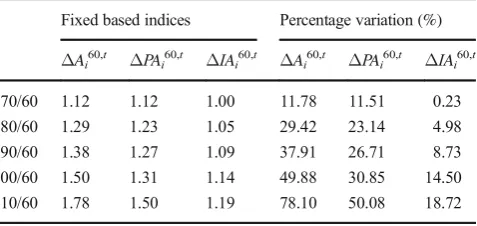
Table 3 shows cumulated changes in accessibility using 1960 as the reference period (ΔA60i ;tÞ, together with the
rela-tive contribution made by changes in population (ΔPAi0,t) and
infrastructure (ΔIAi0,t). Values are expressed as the arithmetic
mean of all provinces (47 NUTS-3). For the overall period between 1960 and 2010, about two thirds of the accessibility increase is due to population change (50.0% out of 78.1%).4 The remainder is due to changes in transport infrastructure. Regarding the accumulated change in accessibility and its
population and infrastructure components in ten year periods, we can see that the increase in accessibility driven by popula-tion and infrastructure is monotonic, as it increases constantly in a cumulative way.
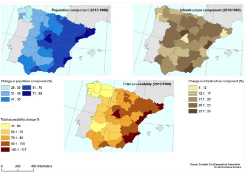
Figure3illustrates the cumulative accessibility change as well as the contribution brought about by the population and infrastructure components for the 2010/1960 period. Comparing the three maps, it is possible to come to a conclu-sion regarding the positive effect that demographic changes and the improvement of transport infrastructure have had on the accessibility of Spanish regions. Regarding the component that is driving the accessibility change, demographic change has a higher weight for all regions in the overall period. This is particularly true for the largest urban regions such as Madrid and Barcelona, where population has constantly increased through immigration flows during this period (Fig.1), as well as for their surroundings provinces, which have benefited from increased accessibility to more dynamic regions.
It is worth noting that some regions register a positive con-tribution of population in their accessibility levels, despite the decline of their population. This happens because regional accessibility levels take into account not only the population within the regional boundaries but also the population of all other regions. Thus, a region that experiences population de-cline in a specific period can still benefit from positive popu-lation changes occurring elsewhere, especially if these chang-es are registered in nearby placchang-es (given the gravity formulation of Eq.1).
Table4shows the change that takes place as the base period is updated every 10 years. The highest overall accessibility increase (18.8%), considering both population and transport infrastructure changes, occurred between 2000 and 2010. This
Table 3 Decomposition of the fixed baseΔA0i;tinto populationΔPA 0;t i and infrastructureΔIA0i;tcomponents
Fixed based indices Percentage variation (%)
ΔAi60,t ΔPAi60,t ΔIAi60,t ΔAi60,t ΔPAi60,t ΔIAi60,t
70/60 1.12 1.12 1.00 11.78 11.51 0.23
80/60 1.29 1.23 1.05 29.42 23.14 4.98
90/60 1.38 1.27 1.09 37.91 26.71 8.73
00/60 1.50 1.31 1.14 49.88 30.85 14.50
10/60 1.78 1.50 1.19 78.10 50.08 18.72
4A similar outcome is achieved using municipalities (LAU regions instead of
decade also registered the highest contribution of population to the accessibility improvement (14.7%) which is in line with population changes shown in Fig.1. Population contribution was particularly important for Madrid and its surroundings as well as for most Mediterranean provinces. In addition, the first two decades (1960–1970; 1970–1980) experienced a relative-ly high accessibility improvement (11.8% and 15.8%, respec-tively), particularly driven by the population change registered in regions such as Madrid, Catalonia or the Basque Country.
For the period between 1980 and 1990 and 1990–2000, accessibility changes were lower due to a modest population increase, especially in most accessible Spanish provinces. On
the other hand, during this period the contribution from trans-port infrastructure outweighs the contribution from population and partly compensates the negative population growth in provinces such as Orense and Vizcaya. If we compare the interannual infrastructure contribution with the number of kilometres constructed in every decade (Table2), we can con-clude that the highest contributions do not fully correspond with the highest investment periods. Instead, transport infra-structure has had the highest impacts in years of network structural changes, such as 1970–1980 when the radial system of highways started to emerge, and during 1990–2000 when this radial structure led to a denser configuration of highways.
6 Conclusions
Historical data on population and transport infrastructure en-ables the analysis of accessibility change over time, while the computation of its separate infrastructure and land use com-ponents offers a much richer explanation concerning the drivers of accessibility improvements. Index number theory has proven very useful to consistently disentangle these com-ponents of accessibility change at a regional level.
Fig. 3 Accessibility changes as a % (2010/1960)
Table 4 Decomposition of interannualΔAit,t+kinto population and infrastructure components
Interannual indices Percentage variation (%)
ΔAit,t+k ΔPAit,t+k ΔIAit,t+k ΔAit,t+k ΔPAit,t+k ΔIAit,t+k
70/60 1.12 1.12 1.00 11.78 11.51 0.23
80/70 1.16 1.10 1.05 15.79 10.43 4.73
90/80 1.07 1.03 1.04 6.56 2.90 3.57
00/90 1.09 1.03 1.05 8.68 3.27 5.31
When applying this methodology for Spain, our results show that changes in transport infrastructure have helped to increase accessibility, although to a lesser degree than demo-graphic changes. In practical terms, this is the result of trans-port infrastructure developments following the actual needs of land use and economic activity during most of the period being analysed, as opposed to being used as an instrument to stimulate growth in less developed zones. The findings for Spain are generally consistent with the results reported in the literature, summarized in section2.
The results suggest that while transport infrastructure can have a long term regional development dimension, policy makers give priority to short-term maximisation of the positive impacts of increasing accessibility. Transport networks linking the main cen-tres of population and economic activity—mainly Madrid and Barcelona in the case of Spain—usually follow radial patterns, which are normally the most efficient solutions in terms of return on investment. The alternative strategy of improving access for areas that lack opportunities would lead to a more equitable evolution of accessibility, but would be far less efficient in eco-nomic terms, at least in the short term. For most countries that are in an important spatial redistribution phase (like Spain during the period), the temptation to concentrate on the short term effects is difficult to avoid. Such investment decisions, however, also lead to a vicious circle: improving the accessibility of the central zones draws new activities to these zones, reinforcing their central role, their attractiveness for additional future investments, and resulting in core-periphery patterns.
It is also clear that priorities, choices and impacts change over time, depending on the level of development already achieved. The returns on improving transport infrastructure in the most accessible regions begin to diminish after reaching a certain point of development. For Spain, given the already high connectivity of Madrid and Barcelona with other locations, increasing their accessibility even more would come at a high cost. The political pressure to invest in less developed regions also increases over time, changing the balance between economic and equity con-siderations in investment decisions.
Our results show that the highest impact of transport infra-structure on accessibility changes does not correspond to the years of greatest network extension, but with years when the network changes structurally. This is particularly due to the development of a radial system of highways, with Madrid as the central point and subsequently, due to the construction of a denser, better connected highway system.
As a general conclusion, the approach and results presented here add to the discussion on the need to integrate transport and land use planning. Our results suggest that the goal to improve accessibility can be better achieved by combining social-economic policies with transport investment decisions. They also provide evidence on the impacts of improving transport networks and their relative weight compared to the impacts of population change for a 50 year period. This allows an ex-post evaluation of the impact of transport infrastructure policies and the quantification of the role of infrastructure and land-use changes in the evolution of ac-cessibility. While the approach can certainly be useful for transport policy in different contexts, it should be kept in mind that the results refer to a specific country (Spain) and a single mode of transport (road). Second order effects, such as congestion, have not been taken into account but may be relevant for other geographic areas.
Appendix
Table5shows a sensitivity analysis to distance decay values
(f ttij in Eq. 1) and internal distance specifications (X in
Eq.3), as well as on the interaction between these two factors. Results are expressed in terms of overall accessibility varia-tion as well as changes due to the evoluvaria-tion of populavaria-tion and transport infrastructure.
The impact of distance decay values was tested by using a power distance decay function and comparing two values of distance decay (α): 1 and 2. Looking at the results forX= 0.33
Table 5 Sensitivity analysis to distance decay value (α), internal travel distance constant used (X)
Fixed based indices
ΔAbi60,t Percentage variation (%)
ΔAbi60,t Δd
PAi60,t ΔIAci60,t ΔdPAi60,t ΔIAci60,t
α= 1 X0.25 1.76 1.50 1.18 76.24 49.53 17.95
X 0.33 1.78 1.50 1.19 78.10 50.08 18.72
X0.5 1.79 1.50 1.19 78.59 50.29 18.86
α= 2 X0.25 1.57 1.41 1.12 57.40 41.43 12.05
X 0.33 1.70 1.45 1.18 70.22 45.45 17.63
(which are the ones used in the paper) we conclude that using a distance decay parameter of 2, slightly decreases the acces-sibility variation from 78 to 70% at the aggregated level, from 50 to 45% regarding the population component, and from 19 to 12% for the infrastructure component. However, the gener-al patterns remain unchanged, since the greater amount of variation in accessibility is due to population change.
Regarding the effect of using different values forXin Eq.3
and the interaction with different distance decay values, we observe a small variation whenα = 1 and slightly higher differences forα= 2.
In general terms, accessibility changes are lower with smaller internal travel distances, as inX= 0.25. This occur because of two joint factors:
& Variations of internal relations in the OD matrix (whenIandj are the same) between to subsequent periods are low, because these are only determined by population changes, since in-ternal distances remain unchanged in the overall period.
& The weight of self-potential is higher using smaller inter-nal travel distances.
Open AccessThis article is distributed under the terms of the Creative C o m m o n s A t t r i b u t i o n 4 . 0 I n t e r n a t i o n a l L i c e n s e ( h t t p : / / creativecommons.org/licenses/by/4.0/), which permits unrestricted use, distribution, and reproduction in any medium, provided you give appropriate credit to the original author(s) and the source, provide a link to the Creative Commons license, and indicate if changes were made.
References
1. Levine J, Garb Y (2002) Congestion pricing’s conditional promise: promotion of accessibility or mobility? Transp Policy 9:179–188
2. Department for Transport (2004) Guidance on accessibility
plan-ning in local transport plans. DfT, London
3. Litman T (2016) Evaluating accessibility for transportation plan-ning. Victoria Transport Policy Institute, Victoria
4. Litman T (2013) The new transportation planning paradigm. ITE J 83(6): 20–28
5. Bertolini L, le Clercq F, Kapoen L (2005/5) Sustainable accessibil-ity: a conceptual framework to integrate transport and land use plan-making. Two test-applications in the Netherlands and a reflection
on the way forward. Transp Policy 12:207–220. doi:10.1016/j.
tranpol.2005.01.006
6. Levine J, Grengs J, Shen Q, Shen Q (2012) Does accessibility
require density or speed? J Am Plan Assoc 78(2):157–172
7. Fujita M, Krugman P, Venables AJ (1999) The spatial economy.
Cities, regions and international trade. MIT Press, Cambridge 8. Fernald JG (1999)BRoads to prosperity^assessing the link between
public capital and productivity. Am Econ Rev 89:619–638
9. Moreno R, Artís M, López-Baso E, Suriñach J (1997) Evidence on
the complex link between infrastructure and regional growth. Int J Dev Plan Lit 12(1&2):81–108
10. Spence N, Linneker B (1994) Evolution of the motorway network
and changing levels of accessibility in Great Britain. J Transp Geogr
2:247–264. doi:10.1016/0966-6923(94)90049-3
11. Geurs KT, van Wee B (2004) Accessibility evaluation of land-use
and transport strategies: review and research directions. J Transp Geogr 12:127–140. doi:10.1016/j.jtrangeo.2003.10.005
12. Gutiérrez J, Gómez G (1999) The impact of orbital motorways on
intra-metropolitan accessibility: the case of Madrid's M-40. J Transp Geogr 30:1–15
13. Holl A (2007) Twenty years of accessibility improvements. The
case of the Spanish motorway building programme. J Transp Geogr 15(4):286–297
14. López E, Gutiérrez J, Gómez G (2008) Measuring regional
cohe-sion effects of large-scale transport infrastructure investments: an accessibility approach. Eur Plan Stud 16:277–301
15. Monzón A, Ortega E, López E (2013) Efficiency and spatial equity
impacts of high-speed rail extensions in urban areas. Cities 30:18– 30. doi:10.1016/j.cities.2011.11.002
16. Kotavaara O, Antikainen H, Rusanen J (2011) Population change
and accessibility by road and rail networks: GIS and statistical ap-proach to Finland 1970-2007. J Transp Geogr 19:926–935
17. Condeço-Melhorado A, Gutiérrez J, García-Palomares JC (2011)
Spatial impacts of road pricing: accessibility, regional spillovers and
territorial cohesion. Transp Res A Policy Pract 45:185–203.
doi:10.1016/j.tra.2010.12.003
18. Geurs K, van Ritsema Eck JR (2003) Evaluation of accessibility
impacts of land-use scenarios: the implications of job competition, land-use, and infrastructure developments for the Netherlands. Environ Plann B Plann Des 30:69–87. doi:10.1068/b12940
19. Gutiérrez J, Condeço-Melhorado A, Martín JC (2010) Using
ac-cessibility indicators and GIS to assess spatial spillovers of
transport infrastructure investment. J Transp Geogr 18:141–
152. doi:10.1016/j.jtrangeo.2008.12.003
20. López E, Monzón A, Ortega E, Mancebo S (2009) Assessment of
cross-border spillover effects of national transport infrastructure plans: an accessibility approach. Transp Rev 29:515–536
21. Koopmans C, Rietveld P, Huijg A (2012) An accessibility approach
to railways and municipal population growth, 1840–1930. J Transp Geogr 25:98–104. doi:10.1016/j.jtrangeo.2012.01.031
22. Axhausen KW, Froelich P, Tschopp M (2011) Changes in Swiss
accessibility since 1850. Res Transp Econ 31(1):72–80
23. Fisher I (1922) The making of index numbers. Houghton-Mifflin, Boston
24. Diewert EW (1992) Fisher ideal output, input, and productivity
indices revisited. J Prod Anal 3:211–248. doi:10.1007/bf00158354
25. Zofío JL, Condeço-Melhorado A, Maroto-Sánchez A, Gutiérrez
J (2014) Generalized transport costs and index numbers: a geo-graphical analysis of economic and infrastructure fundamentals.
Transp Res A Policy Pract 67:141–157. doi:10.1016/j.
tra.2014.06.009
26. MFOM (2014) Los transportes, las infraestructuras y los servicios
postales en España: Informe Anual 2013. Ministerio de Fomento, Madrid
27. Stelder D, Groote P, de Bakker M (2013) Changes in road
infra-structure and accessibility in Europe since 1960. Tender reference nr 20112 CE.16.BAT.040. Final Report
28. Hansen WG (1959) How accessibility shapes land-use. J Am Inst
Plann 25:73–76. doi:10.1080/01944365908978307
29. Rich D (1980) Potential models in human geography. Norwich,
Report Number, 26
30. Condeço-Melhorado AM, Demirel H, Kompil M, Navajas E,
Christidis P (2016) The impact of measuring internal travel dis-tances on self-potentials and accessibility. Eur J Transp Infrastruct Res 16(2):300–318
31. Konüs AA (1924) The problem of the true index of the cost of
living. Transp Econ 7(1939):10–29
32. Maroto A, Zofío JL (2016) Accessibility gains and transport infra-structure in Spain: a productivity approach based on the Malmquist index. J Transp Geogr 52:43–152. doi:10.1016/j.jtrangeo.2016.03.008