R E S E A R C H
Open Access
Image enhancement using local intensity
distribution equalization
Sanparith Marukatat
Abstract
This paper proposes a local intensity distribution equalization (LIDE) method for image enhancement. LIDE applies the idea of histogram equalization to parametric model in order to enhance an image using local information. It reduces the amount of computational resources required by traditional method like the adaptive histogram equalization, but allows enhancing detail similar to the latter technique. Integral image was used to efficiently estimate local statistics needed by the parametric model. This data structure drastically reduces the computational cost especially for megapixel image where a large local window is preferred. It should be noted that, with a large local window, the intensity distribution could contain multiple peaks. LIDE can nicely handle such complex distribution via mixture of parametric models. To speed-up the mixture parameter estimation, we propose an EM algorithm that is also based on the integral image data structure. Experimental results show that LIDE produces an enhanced image with greater detail and lower noise compared to several existing methods.
1 Introduction
Histogram equalization (HE) is a widely used image enhancement technique. It increases the contrast of an image by transferring each grayscale value to a new one via the cumulative distribution function derived from the intensity histogram. For certain images containing varying lighting conditions, or those whose local detail is impor-tant, the global contrast enhancement by HE could be insufficient. Local contrast enhancement can be done by applying HE on the histogram computed in local win-dow around each pixel. This is calledlocal or adaptive histogram equalization(AHE) [1].
AHE is a computational intensive procedure even on today’s computer. Block-based HE is generally used to cut down the computational cost. Pizer et al. [2] apply block-based HE first to some locations in the image. Then an interpolation is used to determine the grayscale of other pixels. This reduces the computational cost at the expense of increasing blocking artifacts. Partially over-lapped sub-block HE (POSHE) proposed by Kim et al. [3] reduces the blocking artifacts. Unfortunately, it does blur the detail of the image along the block boundaries as well. Lamberti et al. [4] suggest that POSHE procedure is, in fact, equivalent to applying the low-pass filter mask on
Correspondence: [email protected]
Image Laboratory, NECTEC, Thailand Science Park, Pathumthani, Thailand
the sub-region histogram. From this observation, they propose to perform POSHE calculation via the binomial filter. The computational cost of this method increases as function of the filter size. Cascade multi-step averag-ing procedure [5] has also been adopted to speed up the POSHE procedure. The resulting process is then faster than the original POSHE, but with the same enhancement capacity. The filtering idea is also used by Gauch [6] and Stark [7]. Both authors use several convolved images to compute local histogram. The computational cost resides mainly in the convolution phase which can be sped up in frequency domain. To speed up the calculation directly in spatial domain, Gonzalez and Woods [8, p. 103] sug-gest to carefully update local histogram since only one column and/or one row of the local window changes as it slides through the image. This idea is implemented later by Wang and Tao [9]. Other speed up techniques include multi-scale HE [10], parallel implementation [11], for example.
HE also suffers from its inability to preserve the bright-ness of the input image. For consumer electronics product such as video surveillance, preserving brightness is essen-tial to avoid generating non-existing artifacts in the output image [12]. To overcome this problem, several research teams propose to partition the global histogram into two parts and apply HE to each sub-histogram independently. Kim [13] and Wan et al. [14] use mean and median of
intensities as partition threshold respectively. Chen and Ramli [15] propose to select the threshold minimizing the absolute mean brightness error between the input and the resulting images. Singh and Kapoor [16] selects the threshold according to the exposure of the image. Recent work by Huynh-The et al. [17] carefully analyzes within-class variance of each interval in order to mini-mize the total squared error of each sub-histogram when equalizing them independently.
The histogram separation idea is further generalized by Chen and Ramli [18] and Sim et al. [19]. These two works rely on a recursive partition of the global histogram, but with different separation criteria. The two techniques produces a partition of the grayscale range into 2r inter-vals where ris set by the user. More generic histogram separation is proposed by Wongsritong et al. [20], and later by Abdullah-Al-Wadud et al. [21] and Ibrahim et al. [22], These authors rely on either peaks or minima of the smoothed global histogram as partition criteria. In practice, we have found that the number of obtained sub-histograms depends on the smoothing procedure applied on the global histogram. Proper size of smoothing filter is needed in order to correctly remove local fluctuations for better enhancement. Menotti et al. [12] propose a more systematic histogram partition based on local discrepancy measures and a dynamic programming algorithm. This requires, however, a larger computational cost.
Other brightness preserving histogram-based enhance-ment techniques are based on histogram matching (HM) procedure. Wang and Ye [23] first search for the ideal target distribution maximizing the entropy while main-taining the average intensity of the input image. Then, HM is used to map the input histogram to this target distri-bution. A similar approach was proposed by Wang et al. [24]. However, the latter chooses the target distribution to be the one minimizing the difference to the uniform dis-tribution subject to the average intensity preservation. In these two techniques, the optimization problem is solved analytically. The overall procedure is then very fast.
In this paper, we propose a variation of HE that can enhance local detail similar to AHE but with lower resources requirement. The basic idea is based on the use of parametric distribution instead of histogram in the equalization procedure. The proposed technique called local intensity distribution equalization (LIDE) relies on parametric cumulative distribution function computed around each pixel to enhance local detail. A data struc-ture called integral image [25] is used to speed up the calculation especially for local statistics. This idea was also proposed recently by Liu et al. [26]. Liu et al. used Gaussian as local parametric model. The reported results showed advantages of this parametric equalization com-pared to existing methods. The authors observed that with a small local window, blocking artifact can be observed
in the output image. A large local window could allevi-ate this problem, but the output will be very similar to that obtained from normal histogram equalization. The test images used in the work of Liu et al. were rather small (512×512 pixels) and the largest local window is equal to the size of the whole image. Experimentally, we have found that when working with a megapixel image, even with a large local window (500×500 pixels), one can still observe blocking artifact. In addition, with a large local window, the intensity distribution becomes more complex. It could contain multiple peaks, in which case the simple model is not adequate.
To handle complex distribution, a mixture model is more appropriate. The proposed LIDE can be used with local mixture model. The combination of LIDE with mix-ture model increases the memory requirement as well as the computational cost. However, compared to LIDE with simple model, it does produce output image with better quality including less blocking artifact. We also propose an EM algorithm that is adapted to take advantage of the integral image data structure for fast calculation.
It is worthy to be noted that the integral image can be used to speed-up the calculation of histogram in local window around each pixel that is needed for AHE as well. Hence, in the following, we shall first present this data structure in Section 2. Then, Section 3 intro-duces the LIDE method with simple probabilistic model (Section 3.1) and LIDE with mixture model (Section 3.2). Section 4 briefly describes how to enhance color images then Section 5 presents the experimental results. In Section 6, we discuss the brightness preserving issue using LIDE. Finally, Section 7 concludes this work.
2 Integral image
Given an imageI, letI(x,y)be the value of pixel at posi-tion(x,y). The integral image ofI, denoted byI, is a two dimensional array in which each position(x,y)contains the sum of all pixel intensities above and to the left of(x,y) inclusive:
I(x,y)= x
x=0 y
y=0
I(x,y). (1)
With this array, the sum of pixel intensities in a local window of size(2d+1)×(2d+1)around a pixel(x,y) can be computed as follows:
f(I,x,y,d) = I(x0,y0)+I(x1,y1)−I(x0,y1)−I(x1,y0)(2)
x0 = max{0,x−d−1} (3)
y0 = max{0,y−d−1} (4)
x1 = min{W−1,x+d} (5)
whereWandHare the width and the height of the input imageI1.
It is straightforward to adapt this procedure to com-pute mean and variance of the local window around each pixel. It should be emphasized that the direct calculation of local sum in the(2d+1)×(2d+1)window around each pixels requires a complexity ofO(4WHd2)forW×H pix-els image. With integral image, the complexity reduces to
O(4WH). This complexity is constant and is independent from the window size. This means that the complexity of calculating the local average of 3×3 window and that of
300×300 window are the same.
The construction of an integral image can be done in a single pass over the input image using an additional accu-mulative arrayS. The following pair of recurrences is used in this calculation:
S(x,y) = S(x,y−1)+I(x,y) (7) I(x,y) = I(x−1,y)+S(x,y) (8) with S(x,−1) = 0 and I(−1,y) = 0. The above con-struction algorithm can be seen as a special case of the wavefront propagation step used in construction of the integral histogram [27].
2.1 Integral image based AHE
We first observe that the histogram of intensities can be expressed as function of several summations, one for each grayscale level. Hence, we can also use the integral image data structure to reduce the computational cost of com-puting local histograms needed by AHE. Indeed, letIlbe the image of grayscale levelldefined as follows
Il(x,y)=1(I(x,y)=l) (9) where1(a)=1 ifais true and 0 otherwise. The histogram h = h0,. . .,h255in the local window of size(2d+1)× (2d+1)around(x,y)can be computed by:
hl= 1 Zf(I
l,x,y,d) (10)
whereIlis the integral image ofIl, andZthe normalizing constant such thatlhl=1.
This approach was also used by Porikli [27] to fas-ten local histograms calculation. However, in that work, the author focused on extracting local histogram with multiple window sizes as signature for object matching.
This integral image based implementation is much faster than direct implementation of AHE, especially for large local window. However, it requires quite large mem-ory since one integral image is needed for each grayscale level. An additional array is needed in the construction process of these integral images. Hence, the memory requirement is an order of O(257WH). For example, to
process an image with 2000× 2000 pixels, about 1 GB
of memory is needed. This corresponds to about 4 M
pixels image which is rather small compared to today’s mobile phone camera. The memory required by this pro-cedure renders it impractical for megapixels images. In return, we can compute local histogram in local window of arbitrary size with the same computational cost. The next section describes the proposed LIDE method that can achieve similar performance as AHE but with much lower memory requirement.
3 Local intensity distribution equalization
The basic idea of LIDE is to use a parametric model instead of the traditional intensity histogram to cut down the memory requirement of AHE. Indeed, a parametric model, e.g., a Gaussian model, is constructed in the local window centered around each pixel(x,y). The cumulative distribution function (CDF) of this model is then used to compute the new grayscale value for the pixel(x,y).
3.1 LIDE with simple model
The CDFs of the two commonly used models namely Gaussian and Laplacian are as follows:
CDFGauss(z,μ,σ)= 1 2
1+erf
z−μ
√
2σ2
(11)
CDFLaplace(z,μ,σ)= 1 2
1+sign(z−μ)
× 1−exp −
√
2|z−μ| σ
(12)
where erf(z) = π20zexp−t2dtis the Gauss error func-tion andμandσare mean and standard deviation (SD) of the sample, respectively.
Given an input image I, LIDE outputs image O is
obtained using the following mapping:
O(x,y)=255×CDF(I(x,y),μ(x,y,d),σ(x,y,d)) (13)
where CDF(z,μ,σ) is CDF of either Gaussian (Eq. 11) or Laplacian (Eq. 12) model, μ(x,y,d)andσ(x,y,d) are local mean and SD in the local window around (x,y). Fortunately, the integral image technique can be used to efficiently compute these values. LetIandI2be the inte-gral image of the input imageIand the squared intensity image, i.e., an image whose value at pixel(x,y)isI2(x,y), we have:
μ(x,y,d)= 1
Df(I,x,y,d) (14)
σ(x,y,d)=min
1 Df
I2,x,y,d−μ2(x,y,d) 1
2 ,σmin
(15)
where functionf as well asx0,y0,x1, andy1are given in
the Eqs. 2 – 6, and σmin is the minimum allowed SD in
order to avoid instability in area of uniform intensity2.
3.2 LIDE with mixture model
It is true that globally, the set of local simple models repre-sent a complex model for intensity distribution modeling. However, with the increasing size of the local window, the simple model may not be sufficient to accurately repre-sent the intensity distribution in each window. A mixture model is more appropriate tool to handle the multimodal distribution. This section describes how to use mixture model in the LIDE method as well as its training proce-dure.
Recall that the probability density function (PDF) of a mixture model withKcomponents is of the form:
p(z)= K
k=1
wkp(z|μk,σk) (17)
where p(z|μk,σk) is the PDF of the component k, and wk is its prior distribution. Two mixture models namely Gaussian mixture model (GMM) and Laplacian mixture model (LMM) are considered in this work. However, the proposed method can also be applied to other mixture model straightforwardly.
The CDF of this model can be computed as follows:
CDFMixture(z) =
z
−∞ K
k=1
wkp(t|μk,σk)dt
=
K
k=1
wkCDF(z,μk,σk)
where CDF(z,μk,σk)is the CDF of each component, e.g., CDFGauss or CDFLaplace. The output image O obtained from the LIDE with mixture model is then given by:
O(x,y)=255× K
k=1
wkCDF(I(x,y),μk(x,y,d),σk(x,y,d))
.
(18)
3.2.1 EM algorithm using integral image
The above mapping function requires the parameters wk,μk,σk k = 1,. . .,Kfor all pixels in the image. Direct calculation of these parameters involves running an EM algorithm on the local window around each pixel in the image. Three nested loops are then needed; one loop over the pixels, one loop for the EM algorithm, and the inner-most loop for computing local statistics in each iteration. Thus, the overall computational cost of direct implemen-tation is huge.
To reduce the computational cost, we shall assume that the K means, μ1,. . .,μK, are shared across all pixels in
the image, i.e.,μk(x,y)= μk,∀k,∀(x,y). This assumption implies that one needs to compute the difference between each pixel intensity and a mean value only once in order to update the SD of all components in every pixel.
Indeed, let μ(kt),k = 1,. . .,K be the sharedK means at iteration tand letw(kt)(x,y)andσk(t)(x,y)be the prior
distribution and the standard deviation of componentk
of pixel(x,y), respectively. Initially, theKmeans are uni-formly distributed between 0 and 255 (μ(k0) = 255k/K). By default, we initializew(k0)(x,y)to 1/Kandσk(0)(x,y) = 255/K.
The posterior probability of componentkof pixel(x,y) orPk(x,y)is computed as:
Pk(x,y)= 1 Zk ×
wk(t)p(I(x,y)|μk(t),σk(t)(x,y)) (19)
withZk a normalizing value to ensure that the posterior probabilities sum up to 1. Given Pk(x,y), the sharedK means are updated as:
μ(t+1)
k =
(x,y)I(x,y)Pk(x,y)
(x,y)Pk(x,y)
. (20)
Once theKmeans,μ1,. . .,μK, are updated, the standard deviations are recomputed via the integral imageDkof the following squared difference imageDk:
Dk(x,y)=Pk(x,y)
I(x,y)−μ(kt+1) 2
. (21)
The SD update equation is as follows:
σ(t+1)
k (x,y)=min
f(Dk,x,y,d) f(Pk,x,y,d)
1 2
, σmin
(22)
wherePkis the integral image of the posterior probability image. The prior probability is also updated fromPk, i.e.,
w(kt+1)(x,y)= 1
Df(Pk,x,y,d), (23)
where Dis given in the Eq. 16. The proposed EM
algo-rithm using integral image is summarized in Algoalgo-rithm 1.
Algorithm 1EM algorithm for LIDE with mixture model
using integral image.
1. Initialization
2. Iterate until convergence
(a) Compute posterior probability image (Eq. 19). (b) Update all means values (Eq. 20).
(c) Compute the squared difference images (Eq. 21). (d) Update SD (Eq. 22) and prior of each
3.3 Complexity
For simple models like Gaussian and Laplacian, two inte-gral images are needed, one to compute the local mean and another one for local SD. In the current imple-mentation, two passes are needed for LIDE with a sim-ple model. The first pass computes the two integral images, and the second one computes the new grayscale value using the local CDF. The computational cost is
then an order of O(2WH). However, this means that
the two integral images are constructed in the same time. Hence, two additional array (S in the Eq. 8) are needed. The memory requirement is thus an order of
O(4WH).
For LIDE, with mixture ofK components, 3K images
of size W × H are needed for storing σk,wk,Pk k = 1,. . .,K. For each component, the standard deviation update (Eq. 22) and the prior update (Eq. 23) require 2 and 1 additional integral images, respectively. As these updates can be done sequentially, the whole process
requires additionalO(4WH) memory at maximum. The
Kmeansμ1,. . .,μK require onlyK floating point values which are negligible compared to the size of the image. The memory requirement of LIDE with mixture model is then an order ofO((3K+4)WH).
The computational cost of this mixture model is domi-nated by the EM algorithm. For each iteration, 4Kpasses over the image are needed for the four steps a–d in the Algorithm 1. The overall complexity is thus an order of
O(4KWHT), withT the number of iterations in the EM algorithm. In practice, ten maximum iterations are used by default.
4 Color image enhancement
For color image, we first apply the enhancement method to its grayscale version. Then use the ratio between the old and new grayscale value to adjust the 3 channels red, green, blue. LetCbe color image withC(x,y).r,C(x,y).g, andC(x,y).b be the red, green, and blue component of the pixel(x,y). We first convert the inputCimage into grayscale imageIas follows:
I(x,y)= 1 3
C(x,y).r+C(x,y).g+C(x,y).b (24)
Let O be the enhanced version of I obtained from an
enhancement method (HE, AHE, LIDE, etc.), andC˜ be
the enhanced version of C. The pixel value of C˜ is
given by:
˜
C(x,y).r = αC(x,y).r
˜
C(x,y).g = αC(x,y).g
˜
C(x,y).b = αC(x,y).b
withα=O(x,y)/I(x,y).
We have also tested other methods such as enhancing the three channels R, G, and B independently or enhanc-ing only the channel V in HSV colorspace, etc. However, these methods do not always preserve the correct color compared to the original image. The method described above is simple, yet produces correct color. Thus, it will be used in the remainder of this paper.
5 Experiments
5.1 Experimental setup
The complexity analysis in Section 3.3 shows that LIDE requires less memory and computational cost compared to AHE. In this Section, we would like to measure the actual improvement of LIDE. In addition, we also consider the quality of the output image when parametric model is used instead of the traditional histogram. To this end, we use photography images from MIT-Adobe FiveK dataset [28]. The size of images in this dataset is quite large, i.e., about 10 megapixels. For these images, the size of the local window was empirically set to 501×501 (d=200). Indeed, a too small local window could also enhance noise whereas a too large window would fail to enhance local detail. The selected size yields good result in many tests for both AHE and LIDE.
Integral image based AHE was used in this experiment. It should be noted that Pizer et al. [2] suggest that in the histogram building process, one should clip large bins, and distribute the count into small bins of the histogram. This procedure, known ascontrast limited AHE (CLAHE), allows reducing noise amplification, especially from uni-form area. In our implementation, we usedrelative dis-counting strategy to clip the local histograms. Indeed, all histogram bins were discounted by the same propor-tion, and the sum of the reduced count was distributed
Table 1Nomenclature of methods evaluated in this work
Technique Reference Brief description
HE [8] Standard histogram equalization
AHE This work Integral image based AHE
LIDE-G This work Parametric local equalization with Gaussian model
LIDE-L This work Parametric local equalization with Laplacian model
LIDE-GMM This work Parametric local equalization with Gaussian mixture model
LIDE-LMM This work Parametric local equalization with Laplacian mixture model
DHE [21] Recursive histogram partition using peaks and valleys
MHE [12] Histogram partition using dynamic programming algorithm
ESIHE [16] Histogram partition using exposure level of input image
HEGMM [29] A Gaussian mixture model is fitted to the global histogram first. Then we use the information from the mixture components to partition the histogram. Parametric equalization is applied to each interval using information from the corresponding Gaussian component
BPHEME [23] Histogram matching using target distribution obtained by maximizing entropy criterion under average intensity preserving constraint
FHSABP [24] Histogram matching using target distribution obtained by minimizing the difference to uniform distribution under average intensity preserving constraint
equally amongst all bins. Five percent discount was used throughout this work.
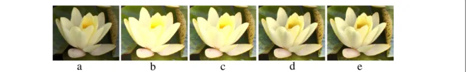
Ten components were used by default for both the Gaussian mixture model (GMM) and Laplacian mixture model (LMM) in LIDE. Hence, LIDE with mixture model would require roughly one seventh of memory needed by integral image based AHE. A less number of compo-nents could reduce the memory requirement as well as the processing time, but it will also reduce the local detail enhancement. Figure 1 shows an example of zoom-in por-tion of the original image in Fig. 2 as well as porpor-tions from images processed by LIDE with LMM using 3, 5, 10, and 20 components. We have experimentally found that 10 components per mixture is a good trade-off between detail enhancement and the resources requirement in several cases.
Four variations of LIDE were considered namely LIDE with simple Gaussian model (LIDE-G), LIDE with simple Laplacian model L), LIDE with GMM (LIDE-GMM), and LIDE with LMM (LIDE-LMM). These four LIDE variations were compared against other existing techniques namely the dynamic histogram equalization (DHE) [21], the multi-histogram equalization (MHE) [12], the exposure-based sub image histogram equaliza-tion (ESIHE) [16], the brightness preserving histogram equalization with maximum entropy (BPHEME) [23], the flattest histogram specification with accurate brightness preservation (FHSABP) [24], and the histogram equaliza-tion with GMM (HEGMM) [29]. These techniques rely on the global histogram. Thus, we shall refer to them asglobal enhancement methods.
For DHE, a smoothing filter of size 3 was used. We applied this filter recursively until the distance between
successive local minima is larger than a predefined value (20 in this experiment). For MHE, the middle value of each interval was used in the discrepancy calculation, and the weight coefficient (the parameterρin [12]) equals to 0.8 was used. In this experiment, we evaluated the number of intervals partition from 5 to 10, and 6–7 intervals were found to be optimal for most images.
HEGMM also relies on a Gaussian mixture model but with different approach from ours. Indeed, HEGMM first constructs a GMM modeling the global histogram of the intensities. Then, it partitions the grayscale range of the input image by analyzing the intersect ion between Gaussian components. For each obtained
Table 2Evaluation results for the first test image (Fig. 2). The size of the original image was 4386×2920 pixels
Technique Entropy EBCM GradMag aPSNR Runtime Mem
(×103) (s)
AHE 5.48 0.88 2.92 12.40 409.9 3 GB
LIDE-G 5.20 0.88 1.88 14.86 2.9 49 MB
LIDE-L 5.34 0.88 2.05 13.52 3.1 49 MB
LIDE-GMM 5.04 0.88 1.84 16.72 181.6 415 MB
LIDE-LMM 5.21 0.88 1.92 15.56 177.3 415 MB
HE 5.45 0.88 1.81 16.68 1.9
DHE 4.92 0.87 1.27 21.60 2.3
MHE 4.92 0.87 1.27 21.24 2.3
ESIHE 5.17 0.88 1.47 17.39 2.1
HEGMM 5.42 0.88 1.69 17.51 2.2
BPHEME 4.88 0.85 1.25 21.70 2.5
interval, HEGMM identifies the dominant Gaussian com-ponent. Once partitioned, HEGMM constructs the map-ping function such that the CDF of the distribution in the output interval is preserved.
Our implementation of HEGMM also relied on the component-wise EM algorithm for mixtures algorithm [30] as used by Celik and Tjahjadi [29]. By default, the mixture model was initialized with 20 components. Then, each component was updated sequentially. The compo-nent whose prior probability falls below 0.001 was dis-carded.
Nomenclature of methods evaluated in this work is summarized in Table 1. Different enhancement tech-niques were carefully implemented in C++ using OpenCV library3. All tests were performed on a MacBook Pro 2.4 GHz Intel Core i5.
5.2 Qualitative results
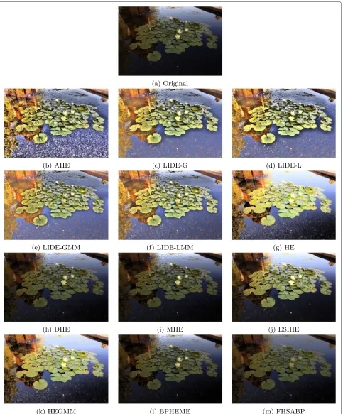
Example 1 is shown in Fig. 2 along with the output from
different enhancement techniques. For this image, AHE and LIDE allow enhancing local detail in the water that cannot be seen in the original image Global enhancement methods can also bring up some detail in the water but not all. In fact, several global enhancement methods barely enhance the detail in this area, since they try to preserve the overall brightness of the input image.
For AHE, all details in the water, on the lotus leafs as well as the ripples on the water seem to be equally enhanced. For LIDE, one can still distinguish between underwater detail and the rest. LIDE with mixture model produces better detail enhancement as can be seen, for example on the lotus flower. The Laplacian model seems to produce a better detail enhancement compared to the Gaussian model for both simple and mixture cases. The output from AHE seems to be the most oversaturated, followed by the output from LIDE with simple model and with mixture model, respectively.
Moreover, one can observe a shadow-like effect around the border of lotus leafs in the output of AHE as well as that of LIDE-G and LIDE-L. Recall that AHE and LIDE enhance each local regions independently. Hence, if the connected regions had distinctive intensities then these techniques will produce transition area between the two regions. This transition area corresponds to the border effect that can be observed. This border effect is less visible in the output of LIDE with both mixture models.
For the memory requirement, AHE needs about 3 GB. LIDE method allows reducing the memory require-ment significantly compared to AHE. Indeed, LIDE with mixture model requires about 415 MB. LIDE with simple model further cuts the memory requirement down to less than 50 MB. The runtime of AHE is almost 7 min. However, it should be emphasized that direct implemen-tation without integral image would require much more
than 7 min to perform the same enhancement. LIDE with mixture of 10 components requires about 3 min. LIDE with simple model needs less than 3 s, that is more than 130 times faster than AHE. The runtime of LIDE with sim-ple model is almost the same as other global enhancement methods. The resources requirement for this example can be found in Table 2.
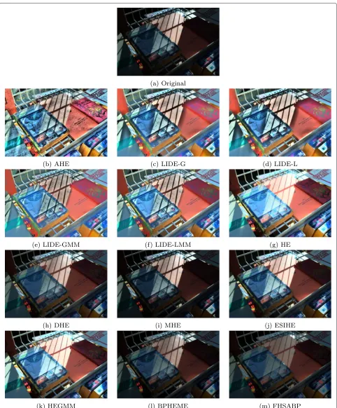
Example 2 is shown in Fig. 3. This image contains
a strong contrast between light and shadow regions. The border effect can be observed again between these regions, especially on the orange cover book in the mid-dle of the image. This effect is more emphasized in the output of LIDE with simple model. LIDE with mixture model produces less border effect, but still more visible compared to AHE. Global enhancement techniques do not yield such artifact, but most of them fail to enhance the detail in this image. In fact, only EISHE and HEGMM successfully enhanced details in the shadow area. They still fail for the bright area. Local techniques, i.e., AHE and LIDE, successfully boosted the detail in both dark and bright regions. They did, however, amplify noise in these regions as well. LIDE produces less noise compared to AHE, especially when using with the mixture model.
For this image, LIDE with mixture model requires mem-ory less than one-seventh of that required by AHE. With simple model, LIDE reduces the memory requirement from almost 3 GB to below 50 MB. This is small enough to fit into today’s mobile device. Moreover, the runtime of LIDE with simple and mixture models are about 3 and 166 s respectively whereas the runtime of AHE is about 410 s. The proposed method is, again, faster than AHE. The resources requirement for this example can be found in Table 3.
Table 3Evaluation results for the second test image (Fig. 3). The size of the original image was 4284×2844 pixels
Technique Entropy EBCM GradMag aPSNR Runtime Mem
(×103) (s)
AHE 5.45 0.87 2.46 12.70 410.8 2.9 GB
LIDE-G 5.29 0.87 1.55 14.00 2.6 46 MB
LIDE-L 5.40 0.87 1.61 12.88 2.8 46 MB
LIDE-GMM 5.08 0.87 1.57 16.20 165.9 395 MB
LIDE-LMM 5.20 0.87 1.57 14.77 165.3 395 MB
HE 5.49 0.87 1.46 14.98 1.5
DHE 4.95 0.87 1.10 18.05 1.6
MHE 4.65 0.87 1.04 17.10 1.7
ESIHE 5.15 0.87 1.21 15.65 1.8
HEGMM 5.29 0.87 1.35 14.85 1.5
BPHEME 4.74 0.84 1.01 19.46 1.8
Fig. 5Staircase effect in the images output from LIDE-G (a) and LIDE-L (b), respectively
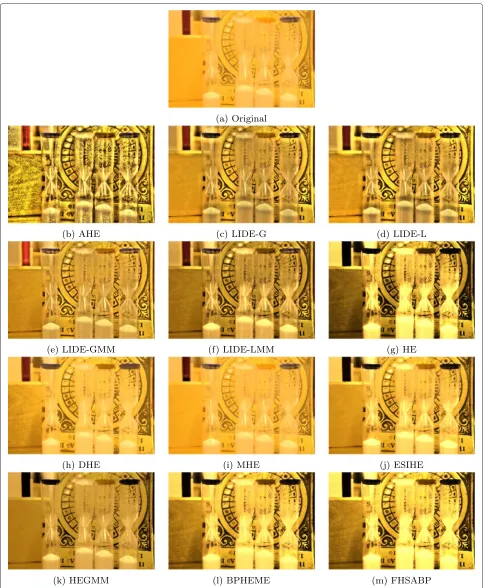
Example 3 is shown in Fig. 4. This image is bright but
with low contrast. AHE yields an oversaturated image as in previous examples. One can observe the border arti-fact in the powder inside the tubes in output images from LIDE with simple model as well as from AHE. LIDE with mixture model seems to be able to better handle this case.
We can also observe astaircase artifactin the left part of the output from LIDE-G and LIDE-L. Figure 5a,b show this portion from Fig. 4 LIDE-G and LIDE-L. In fact, this staircase artifact happens when LIDE is used with sim-ple model, especially in the region with a low variation of intensities. Increasingσminin the Eq. 15 could allevi-ate this problem. However, the local detail in other regions will also be smoothened.
Interestingly, BPHEME and FHSABP that try to pre-serve brightness does overly brighten up the tubes in the foreground. Some local detail in the background seems to be enhanced by these methods as well. For this exam-ple, the output from LIDE seems to be flatter compared to these techniques. The resource requirement for this example can be found in Table 4.
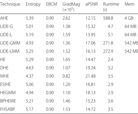
Table 4Evaluation results for the third test image (Fig. 4). The size of the original image was 5010×3336 pixels
Technique Entropy EBCM GradMag aPSNR Runtime Mem
(×103) (s)
AHE 5.39 0.90 2.62 12.15 588.8 4 GB
LIDE-G 5.01 0.90 1.38 15.32 4.7 64 MB
LIDE-L 5.19 0.90 1.59 13.95 5.1 64 MB
LIDE-GMM 4.93 0.90 1.36 17.06 271.8 542 MB
LIDE-LMM 5.25 0.90 1.52 16.13 272.9 542 MB
HE 5.29 0.90 1.65 14.47 2.4
DHE 4.63 0.90 1.07 19.24 3.2
MHE 4.37 0.90 0.82 21.48 3.5
ESIHE 5.06 0.90 1.20 16.81 2.9
HEGMM 4.94 0.90 1.10 18.13 2.9
BPHEME 5.21 0.90 1.46 15.23 3.6
FHSABP 5.17 0.90 1.53 14.72 3.5
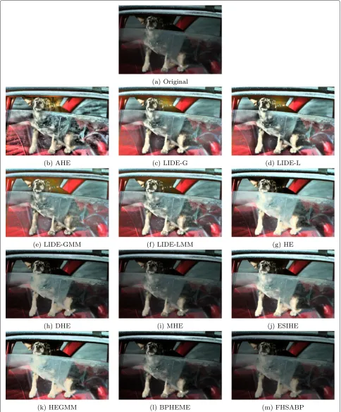
Example 4 is shown in Fig. 6. For this image, all local
enhancement methods amplify noise in the dark area of dog’s ear inside the car. In this case, the ear shape enhanced by AHE seems to be the best. The output from LIDE in this area seems to be pure random noises. Other global enhancement methods do not produce such arti-facts but they do not increase the detail neither on the car’s window nor inside the car. The resources require-ment for this example can be found in Table 5.
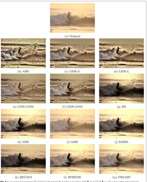
Example 5 is shown in Fig. 7. This image contains a
bright area of the sky on top. AHE performs poorly on this area. Indeed, it amplifies local noises significantly as can be seen in Fig. 7b. LIDE with simple model produces a staircase effect on this area as well. We have experimen-tally found that, generally, the staircase effect appears on a region with uniform intensity. Adjusting the size of the local window could potentially alleviate this problem. It is, however, beyond the scope of this work. Fortunately, working with local mixture model can also resolve this artifact problem. In fact, LIDE with mixture model does not amplify local noise either. Global methods failed to enhance detail in the wave and in the splashing water. The resources requirement for this example can be found in Table 6.
5.3 Quantitative results 5.3.1 Evaluation measures
Entropy. Apart from the visual inspection, we also
com-puted some objective measure to assess the the quality of the enhanced image. Followed the work of Singh and Kapoor [16], the entropy was used to measure the quality of the equalization procedure:
H(I)= − 255
l=0
PI(l)logPI(l) (25)
where PI is the histogram of intensity derived from the imageI. Flatter distribution would correspond to higher entropy.
EBCM. High entropy does not imply better local
Table 5Evaluation results for the fourth test image (Fig. 6). The size of the original image was 3068×2048 pixels
Technique Entropy EBCM GradMag aPSNR Runtime Mem
(×103) (s)
AHE 5.46 0.81 3.02 12.52 180.2 1.5 GB
LIDE-G 5.32 0.81 2.17 13.28 2.0 24 MB
LIDE-L 5.41 0.81 2.31 12.11 1.8 24 MB
LIDE-GMM 5.11 0.81 2.17 15.75 94.3 204 MB
LIDE-LMM 5.31 0.81 2.21 14.12 97.9 204 MB
HE 5.52 0.81 1.96 13.49 0.8
DHE 5.11 0.81 1.67 15.94 0.8
MHE 4.91 0.81 1.45 17.40 0.8
ESIHE 5.41 0.81 1.81 13.88 0.9
HEGMM 5.43 0.81 1.91 13.70 0.9
BPHEME 4.97 0.78 1.59 15.72 1.0
FHSABP 4.89 0.79 1.41 18.65 0.8
detail enhancement, previous works rely on the
edge-based contrast measure (EBCM)[29, 31]. EBCM is defined as function of the following edge-based contrast:
c(x,y)= |I(x,y)−e(x,y)|
|I(x,y)+e(x,y)| (26) where
e(x,y)=
(i,j)∈Neigh(x,y)I(i,j)mI(i,j)
(l,k)∈Neigh(x,y)mI(l,k)
with Neigh(x,y) the set of neighbor pixels of (x,y), and mI(x,y) is the gradient magnitude at pixel (x,y). The EBCM of an imageIis given by:
EBCM(I)=
(x,y)
c(x,y) (27)
Image with higher contrast is expected to have larger EBCM value.
GradMag. Experimentally, we have found that in several
cases EBCM produces similar values that can be hardly distinguished. Thus, in this work, we consider another measure that is theaverage of gradient magnitude. Indeed, good local enhancement technique should increase the magnitude of edges in the output image. It is true that high gradient magnitude could correspond to noise. Besides, we have observed that local enhancement techniques tend to amplify noise. Hence, we also consider measuring the noise level in the output image as described below.
aPSNR. The classical noise level measuring is thepeak
signal-to-noise ratio (PSNR) that is computed from the mean squared error (MSE) between the original noise-free image and the processed image. Low noise image would
correspond to high PSNR value; noisy image would have low PSNR.
It should be noted that PSNR cannot always distinguish noise injection from an enhancement, supposing that we slightly shifted the intensity of all pixels in a black image uniformly toward 255. In this case, we did not introduce any noise into the image. However, the resulting image will have high MSE, thus low PSNR value as if we inject some noise with large amplitude into the original black image. Hence, PSNR does not measure only the noise level in the processed image but also its difference from the orig-inal image. As local enhancement techniques do not aim at preserving the intensity of the original pixels, the out-put image could have high MSE when compared to the input image. This does not necessarily mean that it has high level of noise as one might expect.
To alleviate this problem, we consider the local mean image as reference instead of the original image in MSE calculation. The resulting MSE will be used to computed theapproximate PSNR (aPSNR)as follows:
aMSE = 1
WH
(x,y)
(I(x,y)−μ(x,y,d))2
aPSNR = 20 log10(255)−10 log10(aMSE) (28)
wheredis the size of local window as in AHE and LIDE calculation. Image with low noise should have low aPSNR as well.
5.3.2 Experimental results
Tables 2, 3, 4, 5, and 6 summarize different measures obtained from the output of enhancement methods for each example as well as their runtime and memory requirement. Global enhancement techniques requires only small amount of additional memory that is less than the size of the input image. Hence, their memory require-ment can be considered negligible.
Table 6Evaluation results for the fifth test image (Fig. 7). The size of the original image was 3040×2014 pixels
Technique Entropy EBCM GradMag aPSNR Runtime Mem
(×103) (s)
AHE 5.43 0.82 4.95 12.00 141 1.5 GB
LIDE-G 5.07 0.81 2.67 15.46 1.2 23 MB
LIDE-L 5.17 0.82 2.97 13.98 1.2 23 MB
LIDE-GMM 4.78 0.81 2.60 18.33 67.2 198 MB
LIDE-LMM 4.94 0.81 2.85 17.02 69.4 198 MB
HE 5.16 0.81 2.93 17.75 0.6
DHE 5.10 0.82 2.47 18.46 0.6
MHE 4.74 0.82 1.83 23.36 0.6
ESIHE 4.79 0.82 2.17 17.96 0.6
HEGMM 4.78 0.81 2.05 19.10 0.5
BPHEME 5.11 0.81 2.37 19.35 0.7
FHSABP 5.04 0.82 2.33 20.26 0.6
The dark intensities are mostly distributed to edges and to noises in the output image. This is why AHE produces image with high noise level. LIDE aims at local enhance-ment also yields high noise level. LIDE-L and LIDE-G yield the second and the third lowest aPSNR in most cases. With mixture model, LIDE outputs higher aPSNR, i.e., lower noise level images. In fact, LIDE with mixture model yields comparable aPSNR as global enhancement meth-ods, even higher in some cases. This is in agreement with earlier visual inspection that LIDE with mixture model produces less speckle noises compared to AHE.
5.4 Discussion
The above examples illustrate that the proposed LIDE with mixture model, especially with LMM, allows enhanc-ing local detail similar to AHE, but with less noise amplifi-cation. It requires much less memory compared to integral image-based AHE. This makes LIDE-LMM practical for megapixel images. We can further reduce the resources requirement by using LIDE with simple model (e.g., LIDE-G or LIDE-L). It can be easily implemented on limited resource devices such as mobile phones. However, it may introduce artifacts such as the blocking and the staircase effects.
We believe that LIDE with mixture model amplifies less noise thanks to the EM-training procedure. Indeed, the EM algorithm spreads the information of each pixel amongst all components. This is similar to the histogram clipping and the redistribution of counts in contrast lim-ited HE.
6 Brightness preservation
For some applications, brightness preservation is a required property in order to avoid abrupt change in
the visual brightness and other undesirable artifacts. Preserving the brightness also prevents us from ampli-fying noises in both too dark and too bright areas. An interesting approach by Wang and his colleagues [23, 24] relies on histogram matching (HM) to transform the CDF of an input intensity distribution to the desired target distribution. The target distribution is obtained from a constraint optimization problem where the constraint is to preserve the average intensity, i.e., the average of the target distribution must match the average intensity of the input image. Wang et al. proposed two methods namely BPHEME [23] and FHSABP [24] that differ on the objec-tive function of the optimization problem. Due to the discrete nature of the histogram, the obtained image could have slightly different average intensity compared to the input image.
The above approach can be applied with LIDE straight-forwardly. We start by computing the target distribution (either BPHEME or FHSABP) using global intensity his-togram. Then HM is used in each local window to map between local histogram and the target distri-bution. We have found that this modified LIDE pro-duces image with brightness level closer to that of input image compared to normal LIDE. However, as the local equalization is performed independently around each pixel, the global intensity preserving property cannot be guaranteed. We are working on a better way to com-bine the intensity constraint with local enhancement method.
Figure 8 shows an image and its output from BPHEME, FHSABP, as well as LIDE with LMM and its constrained version using BPHEME and FHSABP target distributions. The average intensity of each image is depicted below it. The normal BPHEME and FHSABP produce average intensity very close to the input image. Constrained LIDE produces larger difference but yield better detail image. In this case, the normal LIDE with LMM overamplifies noise in the dark area at the bottom of the image. By constrain-ing the output to preserve the brightness, the visibility of these noise can be reduced.
Fig. 8An example of image from MIT-FiveK dataset (a) and the outputs from several enhancement techniques;bLIDE-LMM with 3 components,
cLIDE-LMM with 10 components,dBPHEMEeconstrained LIDE-LMM-BPHEME with 3 components,fconstrained LIDE-LMM-BPHEME with 10 components,gFHSABPhconstrained LIDE-LMM-FHSABP with 3 components,iconstrained LIDE-LMM-FHSABP with 10 components
7 Conclusion and future works
This paper proposes a variation of the adaptive his-togram equalization technique called LIDE that is based on parametric model instead of the traditional his-togram of intensities. This allows drastically reduce the memory requirement. We also propose an efficient implementation of an EM algorithm for LIDE with mix-ture model. Experimental results show that it is more than 2 times faster than a carefully implemented AHE. We believe that the integral image based EM algorithm could be applied to other tasks involving mixture model such as the GMM background modeling [32] in video processing. LIDE with mixture model, especially LMM, produces image with clear detail and less speckle noise com-pared to AHE. It is true that local enhancement meth-ods may not be suitable for all cases. However, we believe that if local enhancement is needed, the proposed method represents a good and interesting alternative to AHE.
It is true that local enhancement could lead to noise amplification. Experimental results suggest that LIDE can handle this problem better than AHE. An interesting method to reduce this artifact is due to Saleem et al. [33]. The idea is to fuse the results from global and local enhancement method. This corresponds to fusing enhancement results from multiple scales. We believe that the mixture model used in LIDE can be extended to han-dle this multi-scale enhancement approach nicely. This is currently under investigation.
Finally, both AHE and LIDE can handle the change in lighting condition to some extent. Indeed, information contained in too dark or too bright areas are not sufficient for correctly enhancing these regions. Noise amplifica-tion can be easily observed on these regions. Brightness preservation constraint could be used to conceal such arti-fact. However, a better way to handle this case would be to fuse information from images obtained under different exposures. We believe that the local mixture model used in LIDE may provide an interesting method for fusioning multi-exposure images. This will be further investigated as well.
Endnotes
1This means that we consider pixels outside the input
image as having zero intensity.
2We have experimentally found that setting
D=(2d+1)2would produce artifacts on border pixels where local window fall out of the input image.
3http://opencv.org
Competing interests
The author declare that they have no competing interests.
Received: 18 August 2014 Accepted: 12 August 2015
References
1. DJ Ketcham, RW Lowe, JW Weber, inProceedings of the Seminar on Image
Processing. Real-time image enhancement techniques, (1976),
pp. 120–125. doi:10.1117/12.954708
2. SM Pizer, EP Amburn, JD Austin, R Cromartie, A Geselowitz, T Greer, Romeny B ter Haar, JB Zimmerman, K Zuiderveld, Adaptive histogram equalization and its variations. Comput. Vis. Graph. Image Process.39, 355–368 (1987)
3. JY Kim, LS Kim, SH Hwang, An advanced contrast enhancement using partially overlapped sub-block histogram equalization. IEEE Trans. Circuit Syst. Video Technol.11(4), 475–484 (2001)
4. F Lamberti, B Monstrucchio, A Sanna, Cmbfhe: a novel contrast enhancement technique based on cascaded multistep binomial filtering histogram equalization. IEEE Trans. Consum. Electron.52(3), 966–974 (2006)
5. B Jähne,Digital Image Processing. (Springer, Verlag Berlin Heidelberg, The Netherlands, 1997)
6. JM Gauch, Investigations of image contrast space defined by variations on histogram equalization. CVGIP: Graphical Models and Image Process.
55, 269–280 (1992)
7. JA Stark, Adaptive image contrast enhancement using generalizations of histogram equalization. IEEE Trans. Image Process.9(5), 889–896 (2000) 8. RC Gonzalez, RE Woods,Digital Image Processing. (Prentice-Hall Inc, Upper
Saddle River, New Jersey, 2002)
9. Z Wang, J Tao, inProceedings of the International Conference on Signal
Processing (ICSP). A fast implementation of adaptive histogram
equalization, vol. 2 (IEEE Beijing, 2006). doi:10.1109/ICOSP.2006.345602 10. Y Jin, L Farad, A Laine, inSociety of Photo-Optical Instrumentation Engineers
(SPIE) Conference Series. Contrast enhancement by multi-scale adaptive
histogram equalization, vol. 4478, (2001), pp. 206–213. doi:10.1117/12.449705
11. CW Kurak Jr., inProceedings of the fourth Annual IEEE Symposium on
Computer-Based Medical Systems. Adaptive histogram equalization: a
parallel implementation (IEEE Baltimore, MD, 1991), pp. 192–199. doi:10.1109/CBMS.1991.128965
12. D Menotti, L Najman, J Facon, A de A Araújo, Multi-histogram equalization methods for contrast enhancement and brightness preserving. IEEE Trans. Consum. Electron.53(3), 1186–1194 (2007) 13. Y-T Kim, Contrast enhancement using brightness preserving bi-histogram
equalization. IEEE Trans. Consum. Electron.43(1), 1–8 (1997) 14. Y Wang, Q Chen, B Zhang, Image enhancement based on equal area
dualistic sub-image histogram equalization method. IEEE Trans. Consum. Electron.45(1), 68–75 (1999)
15. S-D Chen, AR Ramli, Minimum mean brightness error bi-histogram equalization in contrast enhancement. IEEE Trans. Consum. Electron.
49(4), 1310–1319 (2003)
16. K Singh, R Kapoor, Image enhancement using exposure based sub image histogram equalization.Pattern Recognit. Lett.36, 10–14 (2014) 17. T Huynh-The, B-V Le, S Lee, T Le-Tien, Y Yoon, Using weighted dynamic
range for histogram equalization to improve the image contrast. EURASIP J. Image Video Process.2014(1), 44 (2014).
doi:10.1186/1687-5281-2014-44
18. S-D Chen, AR Ramli, Preserving brightness in histogram equalization based contrast enhancement techniques. Digit. Signal Process.14, 413–428 (2004)
19. KS Sim, CP Tso, YY Tan, Recursive sub-image histogram equalization applied to gray scale images. Pattern Recogni. Lett.28, 1209–1221 (2007) 20. K Wongsritong, K Kittiyaruasiriwat, F Cheevasuvit, K Dejhan, A
Somboonkaew, inProceedings of the IEEE Asia-Pacific Conference on Circuits
and Systems. Contrast enhancement using multipeak histogram
equalization with brightness preserving (IEEE Chiangmai, 1998), pp. 455–458. doi:10.1109/APCCAS.1998.743808
21. M Abdullah-Al-Wadud, H Md Kabir, MAA Dewan, O Chae, A dynamic histogram equalization for image contrast enhancement. IEEE Trans. Consum. Electron.53(2), 593–600 (2007)
22. H Ibrahim, NSP Kong, Brightness preserving dynamic histogram equalization for image contrast enhancement. IEEE Trans. Consum. Electron.53(4), 1752–1758 (2007)
23. C Wang, Z Ye, Brightness preserving histogram equalization with maximum entropy: a variational perspective. IEEE Trans. Consum. Electr.
24. C Wang, J Peng, Z Ye. Flattest histogram specification with accurate brightness preservation.IET Image Process.2(5), 249–262 (2008) 25. P Viola, MJ Jones, Robust real-time face detection. Int. J. Comput. Vis.
57(2), 137–154 (2004)
26. Y-F Liu, J-M Guo, B-S Lai, J-D Lee, inICASSP. High efficient contrast enhancement using parametric approximation (IEEE Vancouver, BC, 2013), pp. 2444–2448. doi:10.1109/ICASSP.2013.6638094
27. F Porikli, inProceedings of the IEEE Computer Society Conference on
Computer Vision and Pattern Recognition (CVPR). Integral histogram: a fast
way to extract histograms in cartesian spaces, vol. 1 (IEEE, 2005), pp. 829–836. doi:10.1109/CVPR.2005.188
28. V Bychkovsky, S Paris, E Chan, F Durand, inThe Twenty-Fourth IEEE
Conference on Computer Vision and Pattern Recognition. Learning
photographic global tonal adjustment with a database of input/output image pairs (IEEE, 2011), pp. 97-104. doi:10.1109/CVPR.2011.5995332 29. T Celik, T Tjahjadi, Automatic image equalization and contrast
enhancement using gaussian mixture modeling. IEEE Trans. Image Process.21(1), 145–156 (2012)
30. G Celeux, S Chrétien, F Forbes, A Mkhadri, A component-wise em algorithm for mixtures. Technical Report 3746 INRIA Rhône-AlpesFrance (1999)
31. A Beghdadi, Le Negrate A, Contrast enhancement technique based on the local detection of edges.Comput. Vis. Graph. Image Process.46(2), 162–174 (1989)
32. C Stauffer, WEL Grimson, inProceedings of the IEEE Computer Society
Conference on Computer Vision and Pattern Recognition (CVPR). Adaptive
background mixture models for real-time tracking, vol. 2 (IEEE, 1999), p. 252 Vol. 2. doi:10.1109/CVPR.1999.784637
33. A Saleem, A Beghdadi, B Boashash, Image fusion-based contrast enhancement. EURASIP J. Image Video Process.2012(1), 10 (2012). doi:10.1186/1687-5281-2012-10
Submit your manuscript to a
journal and benefi t from:
7Convenient online submission
7Rigorous peer review
7Immediate publication on acceptance
7Open access: articles freely available online
7High visibility within the fi eld
7Retaining the copyright to your article