Machine Learning and Predictive Analysis of Fossil
Fuels Consumption in Mid-Term
Mahmood Amerion
1, Mohsen Amerion
2,* ,Mohammadmehdi Hosseini
1and Abdorreza Alavi
Gharahbagh
11. Faculty of Electrical and Computer Engineering, Azad University, Shahrood Branch,P.O.BOX 43189-36199 2. Faculty of Science, Engineering and Technology, Swinburne University, PO Box 218 Hawthorn, Victoria, 3122 Australia
Abstract
In economies that are dependent on fossil fuel revenues, Realization of long-term plans, mid-term and annual budgeting requires a fairly accurate estimation of the amount of consumption and its price fluctuations. Accordingly, the present study is using machine learning techniques to predict the usage of fossil fuels (Diesel, Black oil, Heating oil, and Petrol) in mid-term. Exponential Smoothing, a model of time series and the Neural Network model have been applied on the actual usage data obtained from Shahroud area from 2010 to 2015. For estimation of predictive value by Neural Network method, the training and testing samples, the highest and lowest errors with a range of 41% -0.89% and 88% -3% for the Mean Absolute Percent Deviation are the most appropriate predictions for Petrol consumption. And in the Single Exponential Smoothing, the forecast rate for each product is estimated on a quarterly as well as monthly basis.
Keywords
:
Parallel Processing, Information Systems, ScalabilityCorresponding author. Email:[email protected]
1. Introduction
The advancement and progress of each country depends on the establishment of cooperation and interconnectedness of the economic sectors, in which fossil fuels play a key role as one of the most important economic issues So that today, fossil fuels
and in general, energy carriers play a key in various economic sectors and sub-sectors. Therefore, fossil fuels are of great importance for consumers, decision-makers and planners due to their value of income, consumption etc. However, with the Received on 29September 2017, accepted on 13 November 2017, published on 28 December 2017
Copyright © 2017Mahmood Amerionet al., licensed to EAI. This is an open access article distributed under the termsof
the Creative Commons Attribution licence (http://creativecommons.org/licenses/by/3.0/), which permits unlimited use, distribution and reproduction in any medium so long as the original work is properly cited.
expansion of cities and geographic areas, urban and economic problems have increased, since, on the one hand, these types of fuels are from non-renewable sources, by passing time, their production is reduced, and on the other hand The dependence of the economy on this sector leads to less attention to other sectors that may be highly productive in terms of income generation. Also, the use of different fossil fuels will cause greenhouse gas emissions and environmental pollutants. In human societies, development can be achieved with the use of more energy, and thus human beings transform their environment into their physical, chemical, biological and social characteristics to achieve development. Today, energy production and utilization policies play a pivotal role in local and regional environmental issues. Therefore, the need to determine the complex relationship of environmental issues with energy carriers has become more tangible. (Abdoli and Yadhqar, 20: 2007)Accordingly, energy security is affected by political, economic and energy price changes, and to mitigate the effects of crises and oil shocks and the problems of dependence on gasoline, oil and gas as transport fuels The use of alternative fuels, such as CNG, could be a good solution, but it should be noted that the use of this alternative fuel could allow all the country's capacities to be considered for the use of non-fossil and renewable fuels. And the use of this fuel does not neglect other areas and it is better to firstly have a fuel basket in the transport sector and to use alternative fuels based on this fuel basket. Regarding the implementation of the CNG replacement plan as a national plan from 2000 to date, it was necessary to address the development of infrastructure including the construction of CNG fuel stations and the conversion and commissioning workshops for dual-fuel vehicles. So far, it has been
completed and evaluated in order to make further improvements. Therefore, considering the importance of fossil fuels and the problems in this area, machine learning as a tool can also predict fuel consumption at different times, so the philosophy of machine learning is that the future is much like in the past. And if we know the past well, we can predict the future with a high approximation. Machine learning duty is to extract and retrieve valuable information from big data. At the beginning of the machine learning process, your company or organization will find problems, and in the end, with the help of artificial intelligence, solutions will be available to solve these problems. Various factors are decisive in this prediction, including seasonal variations, climatic conditions, demand, types of products and consumption areas (e.g. transportation, agriculture and livestock, production and industry, factories, energy, etc.).Therefore, the use of available data for future forecasting will be of great help to our behavior towards consumption as well as to implement constructive plans to reduce fuel consumption and its purposefulness. For this reason, as little academic research has been done in this field, the purpose of this study is to use the data available in the transport company of petroleum products. The consumption of products in the Shahrood region from 2010 to 2015 and the answer to the question that, how do fossil fuels consumption can be predicted by machine learning? It should be noticed that the timing in this study is based on Persian calendar as for the years, research data are between 1389 and 1394 which is almost equal with the period of 2010 and 2015. Also for the monthly basis, Farvardin which is the first month of the year and also is the first month of spring season in Persian calendar, is almost equal with March and is similar for the other month.
2. Subject topics1
The success of neural networks as a powerful tool for analyzing data has attracted the attention of economists in this way and in the late 80's various models have been developed to predict economic variables. In the field of predicting economic variables by artificial neural networks and comparing the results of other models, different studies have been done. Accordingly, foreign studies conducted in this area include:
Longo,C and his Colleagues (2007) ,”Evaluating the Empirical Performance of Alternative Econometric Models for Oil Price Forecasting” Econometric models were used to predict crude oil prices in the
three main groups of structural and mixed models, time series, and financially, and then to evaluate the ability to forecast prices by each of these models with different horizons of time (annually, seasonally, monthly and daily). The results of the studies indicate that the financial error correction models do not provide accurate forecasts of the crude oil price point, and the proposed models of Longo, entitled "mixed models", according to the data and evaluation criteria used in the study, they were recognized as a superior model.
range regression methods for prediction of tractor fuel consumption”. The study concluded that predicting fuel consumption in the tractor could lead to the selection of the best conservation practices for farm equipment. Using an Artificial Neural Network model (ANN), six training algorithms for predicting fuel consumption were adopted. The highest performance for a hidden double layer, each containing 10 neurons, was obtained using the Levenberg-Marquardt training algorithm. The results showed that ANN and stepwise regression model showed similar detection coefficient (𝑅2= 0.986 𝑎𝑛𝑑 𝑅2= 0.973, respectively). While ANN was given relatively better prediction accuracy (𝑅2= 0.938) compared to step-by-step regression (𝑅2 = 0.910), one of the benefits of ANN was the model of the integration of load and torque conditions in the form of a model.
Adrien Boiron and others, “Predicting Future Energy Consumption"(2012), have expressed Load forecasting for the electrical industry is an important step in planning and application, especially by increasing the use of these industries. The purpose of the project is to accurately predict the hourly consumption rate (in kilowatts) in 20 regions using 4 year data and temperature data 11 at different stations. Several linear return models have been developed and provide reliable prediction of energy load with less than 5% error. During the data process, it significantly eliminates the power outages caused by the power outage and a sudden jump to the loaded part.
Eva Ostertagova (2012), "Forecasting using simple exponential smoothing method ". In this paper, the relatively simple, yet powerful and all-round technique for predicting the time series data_ exponential smoothing is described. So that the accuracy of the SES method depends heavily on the ALPHA which is the smoothing parameter. 'ALPHA' used To determine the optimal value in the article, a traditional optimization method based on the lowest mean absolute error value, the mean absolute percent error and the mean square error.
FatihTas and others (2013), have been studied "Forecasting of daily natural gas consumption on regional basis in Turkey using various computational methods" Accordingly, a limited number of computational methods have been used to estimate accurately the short-term energy demand using 4-year-old gas consumption volumes. Among these methods, the ANN and time series are widely used for short-term estimation of natural gas in certain areas of Turkey. Therefore, although the data has been small, the proposed algorithm works to predict
short-term natural gas consumption and produces encouraging and meaningful results for future energy investment policy.
Girish Kant & Kuldip Singh Sangwan (2015), Have been studied ” Predictive Modeling for Energy Consumption in Machining using Artificial Neural Network”, The results are very close to the experimental values with only 1.5% errors which represent the accuracy of the model.
Jolanta Szoplik (2015), Have been studied” Forecasting of natural gas consumption with artificial neural networks” In this study, the results Projected gas demand forecast using artificial neural networks is provided. Design and training of the MLP model using descriptive data on natural gas consumption in Szczecin (Poland). High-quality MLP networks were used to provide gas consumption prediction for additional input data, which had not previously been used in the training process. It has also been found that the MLP22-36-1 model can be successfully used to predict gas consumption per day of the year and every hour of the day.
From internal studies conducted in this regard, we can mention the work of Golestani and others (2012) who have compared the" prediction of VAR, ARIMA and ANN models for OPEC global oil demand". The results show that the VAR model with an error rate of 6% for the mean squares errors, 19% of the mean absolute error value and 5% of the mean absolute percent error is the most suitable prediction for the global demand for OPEC oil. Therefore, according to the VAR method, demand for OPEC oil is projected to increase in the 2012. The prediction for global oil demand for the organization by 2015 suggests that demand for OPEC oil is rising, but the pace of this increasing trend will slow down in 2014.
Appendix A. Materials And Methods
A.1.Time Series Prediction Model: Simple Exponential Smoothing
In many cases, a simple exponential smoothing is used to predict future values of the time series. Exponential Smoothing method is useful for those time series that there are no definitive and periodic changes and also there is a lot of use for predicting future consumption. In this method, like the averaged moving weight method, different weights are given to the data of different periods, so that the weights follow a descending geometric progression. In this method, the maximum weigh allocates to the latest consumption period and if we go back to the later
periods, weights are reduced exponentially. In the formulation of this average, the highest weight is given to the newest observation, and the lowest weight is given to the oldest. Also, in this method, unlike the moving average weighted, only a few past periods are not fixed, but all courses are considered in the calculation of the forecast. This method uses the prediction made in the previous period and corrects its error bias to predict the future period (Azar and Momeni, 328: 2009). However, the exponential smoothing formula is as follows:
Ft+1= α. At+ (1 − α)Ft .
Due to the existence of these return relationships between Ft and Ft+1 , Ft+1 can be represented in another way, as in (A.2)
It is clear that in this form of relationship expression, exponential smoothing assigns the highest weight to Atand less weights to previous observations.
In addition, this relationship is a simple way, because maintenance of data before the 't' period is not required to estimate the demand for the next period.
All that is required is Atand the previous prediction is Ft. The formula of exponential smoothing can be expressed as (A.4):
Ft+1= Ft+ α. (At− Ft). (A.4)
In the above relation:
• Ft+1: The prediction rate of the next period
• Ft : Forecast the previous period • a : constant coefficient of smoothing • At : Amount of previous period
Forecast of the next period = Forecast of the previous period + α. (Forecast error of previous period).
Also, in the simple exponential smoothing formula, 'α' (ALPHA) is called the constant coefficient of smoothing or smoothing, and its value is between
zero and one. In what amount that the Alpha be closer to zero indicates the worthless value of real consumption data and, as close as possible to one,
1 t
1
t 11
2 t 2t
A
A
A
F
1 t
1
t 11
t 2t
A
A
A
F
(A.1)
(A.2)
(A.3)
.
indicates the value of actual consumption data. Sometimes the value of 'a' is obtained empirically from the test and error method on a bunch of past
data, and the amount of a, which results in less error, is more favorable.
A.2.Neural Network Model
The simple shape of the neural network is usually composed of the input layer, the hidden layer, and the output layer. The input layer is a transmitter layer and a device for data acquisition. The output layer contains values predicted by the network, which represent the output of the model. The hidden hub, which consists of processor neurons, is the place where data is processed. The number of layers and the number of neurons in each hidden layer is determined by experiment and error (Asghari Moghadam and his Colleagues, 3: 2009). Accordingly, the input layer contains input variables, including 𝑥1،𝑥2، 𝑥3،…،𝑥𝑛, and ‘n’ also represents the number of variables. The output layer also contains many output variables, such as 𝑦1،𝑦2،𝑦3، … 𝑦𝑛,
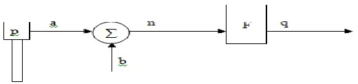
each input ‘x’ is connected to a ‘y’ in output. In fact, the neural network is a collection of neurons interconnected in different layers that send information to each other. Artificial neurons are simple information processing units, so a large number of these neurons form a neural network. However, the structure of a single-entry neuron can be seen in the figure below. The ‘p’ and ‘q’ scalars represent the input and output respectively. The effect of ‘p’ on ‘q’ is determined by the amount of scalar ‘a’. The other input, which is a constant value of 1, is multiplied by a sentence with b, then summed with ‘a p’. This sum is a net input of ‘n’ for the stimulus function ‘f’. Nevertheless, the output of the neuron is defined by the following equation:
q = f (ap + b)
Figure 1. Single imported nerve structure
What is important and should pay attention to is the effect of the sentence b (bias). This sentence can be considered as the weight a, with the notion that b reflects the effect of constant input on neuron. It should also be noted that the parameters ‘a’ and ‘b’ are configurable and the stimulus function f is also selected by the designer. Also, depending on this choice and the type of learning algorithm, parameters ‘a’ and ‘b’ are set. Learning means that ‘a’ and ‘b’ change in such a way as to match the input and output relation of the neuron to a given target. (Golestani and others, 153: 2013).
Therefore, the ability to learn from input data is the most important advantage of the neural network, as it provides an acceptable output for previously unseen input data and the importance of this factor in prediction is high. Also, the ability to run neural networks on parallel computers has added to the importance of this method, but given the advantages, the model also has weaknesses, the most important of which is data constraints. In addition, there is no definite rule for the sample size required for a problem (Yusefi Zonur and Manhaj, 35: 2011).
AppendixB. Performance Evaluation
Considering that different predictive methods (quantitative) have different accuracy, to determine the appropriate method, we need to look at the
should minimize the forecast error. Accordingly, in the neural network model, the most important indicator for predicting error is the mean absolute
percent deviation. This criterion can be shown according to the following relationships:
MAPD= ∑Ni=1 |At−Ft|
∑Ni=1At .
In this regard, At− Ftis the difference between the actual consumption and consumption forecast, and ∑𝑁𝑖=1𝐴𝑡 represent the total of actual consumption.
AppendixC. Data And Information
In this study, the daily, monthly and annually time series data for the consumption of fossil fuels (Petrol, Diesel, Heating oil and Black oil) during 2010 to 2015 was collected through an interview from
Shahroud Transport Company. Based on this, Exponential Smoothing and Neural Network method have been used to predict the consumption of fuel products.
AppendixD. Estimate The Forecast Model
D.1.Predict With Simple Exponential Smoothing Method
Given that the Exponential Smoothing method is
one of the most widely used methods for
predicting the future, it is one of the simplest
and most commonly used prediction methods,
and is also the basis for other prediction models.
Therefore, the consumption of 48197 fuel
products monthly and quarterly is predicted
using Power BI software from 2010-2018. (The
graphs are based on Persian calendar
between
1389 and 1397 which are almost equal with
the period of 2010 and 2018).
The results are
presented in the form of charts:
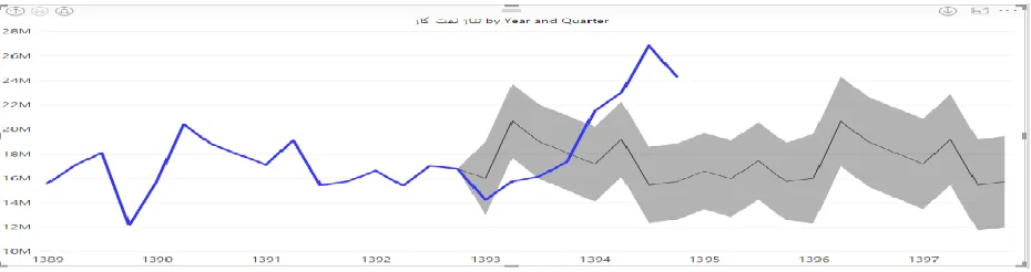
Figure 2. Diesel forecast by quarter
Regarding to actual consumption from 1393 to 1397 (almost equal to 2014 to 2018), Future consumption levels (in spring, summer, autumn, winter) will have ascending and descending trend, so that by 95% it can be said that this can be less or more. Also, in the period of 1393-1394 and 1396-1397, Diesel consumption is expected to be the highest. On the other hand, the amount of gas oil consumption in the
Figure 3. Diesel forecast, monthly
According to Figure 3, the amount of Diesel consumed in the future, which has been surveyed on a monthly basis, has been measured since 1393,
indicating that initially consumption decreased over a short period of time And then the it will projected an ascending-descending trend.
Figure 4. Black oil forecast by quarter
According to Fig. 4, it is noticeable that, the amount of Black oil consumption is decreasing, because according to the studies carried out in 1389, the most consumers were furnace burners, and on the other
hand, changing government's policies towards consumer and compel them to alter their fuel to gas burning, has pushed the demand towards less consumption.
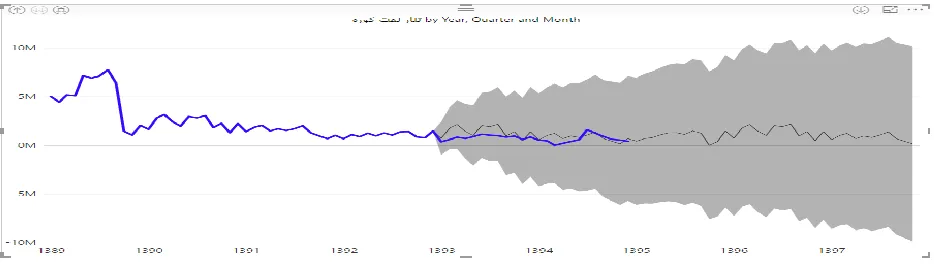
Figure 5. Black oil forecast, monthly
Figure 6. Heating oil forecast by quarter
The consumption of Heating oil in seasons shows that demand (consumption) is rising from the beginning of the third quarter to the middle of the fourth quarter, as the consumer needs this fuel due to
the beginning of the cold weather in Shahroud area and it has been declining since the middle of the fourth quarter because consumer fill their tankers and the weather goes warmer.
Figure 7. Heating oil forecast, monthly
The amount of heating oil consumption per month shows that this fuel can be predicted in the future with an increasing-decreasing trend, so that by about
95% it can be said that this amount may be less or more.
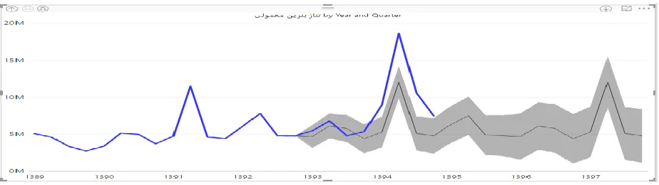
Figure 8. Petrol forecast by quarter
In second quarter of 1391 and 1394 the consumption experienced a significant increase, because during this period volume of summer travel is high, it has a key role in increasing the consumption of Petrol. And on the other hand, according to an interview with oil
Figure 9. Petrol forecast, monthly
As can be seen from the prediction graph, there are some fluctuation in the Petrol consumption and the period with the highest consumption are obvious. As Power BI software is unable to display predictive mathematical relations and only displays the results in graphs, for more precise examination and estimation of errors, the results of the time series prediction of the simple Exponential Smoothing method on Petrol consumption as one of the fuel products calculated in MALTAB Software and then
generalized to other products. In order to analyze and evaluate the prediction using this method, the data of different months are investigated in a time series, so that a pattern for January, February, March,... and December is considered. And the forecast of the Petrol consumption on a monthly basis under consideration is based on the formula of the Time series method, as shown below, based on the forecast rate of two months ago and the forecast of the previous month:
0 1 1 2 2
i i i
Y
y
y
According to the relation (D.1), 𝑦𝑖−1 is the prediction of the previous month and 𝑦𝑖−2 is the prediction of two months earlier.
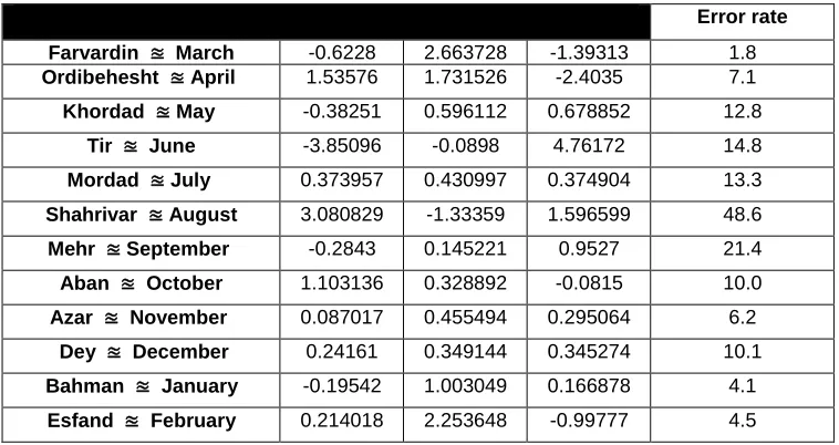
Table 1. The coefficients obtained for the Petrol consumption in the formula (D.1) on a monthly basis.
Error rate
March ≊
Farvardin -0.6228 2.663728 -1.39313 1.8 April
≊
Ordibehesht 1.53576 1.731526 -2.4035 7.1 May
≊
Khordad -0.38251 0.596112 0.678852 12.8 June
≊
Tir -3.85096 -0.0898 4.76172 14.8 July
≊
Mordad 0.373957 0.430997 0.374904 13.3 August
≊
Shahrivar 3.080829 -1.33359 1.596599 48.6 September
≊
Mehr -0.2843 0.145221 0.9527 21.4 October
≊
Aban 1.103136 0.328892 -0.0815 10.0 November
≊
Azar 0.087017 0.455494 0.295064 6.2 December
≊
Dey 0.24161 0.349144 0.345274 10.1 January
≊
Bahman -0.19542 1.003049 0.166878 4.1 February
≊
Esfand 0.214018 2.253648 -0.99777 4.5
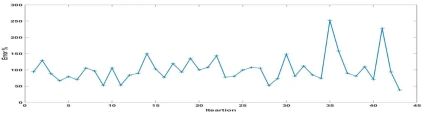
Graph 1. Prediction error
The results of Table 1 show that by using the time series method, it is possible to predict the average Petrol consumption in January with the lowest error of 1.8% and in September with the highest error of
48.6%. The error rate is also used by the mean absolute percent deviation (MAPD) as previously noted.
D.2.Prediction By Neural Network Approach
For prediction using the neural network method, which is one of the methods of machine learning, the daily and monthly data of Petrol consumption as one of the fossil fuels and generalization of other fuels from 2010 to 2015 are classified. However, the construction of neural networks according to studies is much longer than designing an estimation of the relationship between variables (regression) in order to predict. Therefore, in designing a neural network, selecting variables as inputs, the network structure should also be evaluated with the best prediction, so that the change in the structure of a network, even if the input variables, output, or sample size do not change, prediction basically changes, Therefore, in order to find the best structure of the network, we must go through test and error. What is evident in this method, like other methods of nonlinear estimation, cannot be guaranteed to achieve absolute minimum. Accordingly, for a given set of inputs and a given network structure, several initial values of different weights must be repeated several times. The weights that are estimated to lead to the lowest Mean Absolute Percent Deviation (MAPD) can be considered as the best possible result for a given set of inputs. Also, to evaluate the performance of other networks, the network structure has to be modified by changing the number of layers and hidden parts, and adding or removing communications between units of different sections of the network. All stages of the estimation process should be repeated in the hope of finding the absolute minimum, and then the results of the estimation of the networks are evaluated by comparing the error rate obtained in each structure. After evaluating and analyzing different networks,
the network will be selected that has the lowest error. Accordingly, to predict consumption by the approach of neural networks, generally used a multi-layer perceptron (MLP). The Feed forward network rule is used to train the neural network. This law consists of two main routes. The first path is called forth and referred to as the path that goes through the input vector into the MLP network and its effects are transmitted through the middle layers to the output layers. The output vector generated in the output layer forms the true MLP network response. In this way, the network parameters are considered constant and unchanged. The second route is known as the back path. In this direction, on the contrary with forth path, the parameters of the MLP network are changed and adjusted. This setting is done in accordance with the error correction rule. The error signal is formed in the network output layer. The error vector is equal to the difference between the appropriate response and the real network response. The error value, after calculation, and through the back path of the output layer is distributed in the network layers throughout the network. We also set the number of hidden layers in this study 8,9,10,11,12 and repeat the number of repetitions in this study, each of which 30 times, and set the error rate as a performance evaluation, because the purpose of the work before Nose is looking for the lowest error with high precision. Because the goal of doing this study is prediction, we are looking for the lowest error with high precision. Therefore, the output of the neural network method with MATLAB Software is described in the following graphs:
1.8 7.1
12.8 14.8 13.3
48.6
21.4
10.0 6.2 10.1
Chart 2. Lowest error rate
To check and analyze the error rate, the lowest error in the Layer 9 can be seen at 34%, and this error rate is acceptable.
Also, the results of the coefficient of determination are shown in the following figure:
Chart 3. Fig. 3. Regression graphs of measured and output values for training, validation and test data sets in the network with 8 hidden layers and Levenberg–Marquardt training algorithm (MATLAB software).
According to Chart. 3, the rate of 𝑅2, which is related to the Normalized Mean Square Error (NMSE), is called the determination coefficient and is calculated as follows:
NMSE=1-𝑅2. (D.2)
𝑅2 shows the change directions of independent and dependent variables, and its value is between zero and one, and the value of one represents the complete match of the data. The zero value for 𝑅2 represents a function that can be expected from the use of the mean real output value d as the basis for predictions. According to Chart (3), the coefficient of
Chart 4. Results from increasing the Repetition
Considering that in this study in order to examine the results 70% of the data were used as training information and 30% of them were tested. Therefore, the results of the actual amount (in millions / liters)
and the amount of the model and the error rate (in percent) for the samples of training and samples of the test is as follows:
Table 2. Actual value and Neural Network Pattern Error of Petrol consumption for the training data
Table 3. Actual value and Neural Network Pattern Error of Petrol consumption for the test data
Sample number
Actual value Model value Error in percent
54 1.487 1.37 7.98 58 3.692 2.19 40.78 47 1.175 2.22 88.69 56 1.545 1.43 7.15 62 4.549 4.22 7.26 55 1.364 1.25 8.33 5 1.19 1.23 3.38 31 1.266 1.09 14.19 Sample
number
Actual value Model value
Error in percent
32 1.252 0.98 21.51 10 1.201 1.38 14.70 11 1.038 1.10 6.18
2 1.444 1.31 9.39 38 2.361 2.34 0.89 63 7.6 4.46 41.36 40 2.323 2.18 6.27
66 2.788 1.02 63.56
61
6.561
2.76
57.89
The results from Table (2) is for training samples and the table (3) for test samples and the results show that the error rate in test samples has increased, even the error rate reached 88%, but on average no more than
a specified number. Also, the error function which used to evaluate the model is mean absolute percent deviation (MAPD).
AppendixD. Conclusion
Considering that each fossil fuels play a significant role in the economy and planning of the country, they must be measured with a higher degree of accuracy, since these fuels are non-renewable, if their consumption levels do not predicted more accurately in the future, they will be disturbed in revenue and consumption decisions. Therefore, it is necessary to accurately predict the rate of use and the amount of demand (consumption) for these fuels. Therefore, in order to predict mid-term consumption, the Exponential Smoothing method is used as one of the methods of Time series prediction and Neural Network method as one of the methods of Machine Learning. The results of the Exponential Smoothing method are initially seasonally and monthly for (Petrol, Diesel, Heating oil and Black oil) using Power BI Software, so the results indicate that the amount of these products will be increasing - decreasing or vice versa. The mathematical results from the review of the Time series for Petrol on monthly basis have shown that in September the forecast of consumption with an error of 48.6 (the highest error rate) was estimated and in April the prediction of Petrol consumption is estimated at 1.8,
which is the lowest error rate. Also, with the Neural Network method, the error rate in the test samples has increased compared to the training samples, so that the highest and lowest errors in the test sample is 88% and 3% respectively, and the least error in the layer 9 has been extracted by 34% which is an acceptable error rate and the correlation is estimated at 95% accuracy, which indicates a strong correlation in this study. Accordingly, according to these findings, Golestani and others who compared the forecast of VAR, ARIMA and ANN networks on the global oil demand of OPEC. The forecast for the global oil demand (as a fossil fuels) forecast by 2015 suggests that demand for OPEC oil is rising, but the pace of this increasing trend will slow down in 2014. Therefore, it can be said that the results of this study coincide with the results of our study that the amount of oil had a decreasing trend. Naghavi Azad has been analyzing the replacement of solar energy with fossil fuels and suggests that in recent years, new technologies can be a factor in replacing solar energy with fossil fuels, which is consistent with our research results, due to the fact that the amount of products has been increasing or decreasing.
PS
This paper is based on the master's thesis.
References
[ 1
] Journal article: Asghari ,M.(2008) Modeling of rain fall rate in Tabriz plain using artificial neural networks. Journal of Agricultural Science, Tabriz University:1-15.
[ 2
] Journal article: Abdoli,M and Yadhqar, A.(2006) Energy, Development and Environment. Iranian Journal of Energy :19-28.
[ 3
[ 4
] Journal article: Chakravorty,U and Tse,K.P.(1999) Transition from Fossil Fuels to Renewable Energy: Evidence from a Dynamic Simulation Model with Endogenous Resources Substitution. Indian Journal of Quantitative Economics.
[ 5
] Journal article: Eva, and Oskar ,O.(2012) FORECASTING USING SIMPLE EXPONENTIAL SMOOTHING METHOD.
Acta Electrotechnica et Informatica: 62–66.
[ 6
] Journal article: Fu,j.(1998)A Neural Network Forecast of Economic Growth and Recession. the journal of economics:51-66.
[ 7
] Journal article: Fatemeh,R and Yousef,A.(2011) Artificial Neural Network and stepwise multiple range regression methods for prediction of tractor fuel consumption. journal homepage:2104-2111.
[ 8
] Journal article: Golestani, S, Ghorgini, Mand Haj Abbasi, F.(2013) Comparison of the ability to predict VAR, ARIMA and Artificial Neural Networks models on Global demand for OPEC oil. Journal of Environmental Economics and Energy
:145-168
[ 9
] Journal article: Girish,K and Kuldip,S.(2015) Predictive Modelling for Energy Consumption in Machining using Artificial Neural Network.ELSEVIER:205-210.
[ 10
] Journal article: Houshyar, M, Hosseini, A and Mesgari, E.(2013) Modeling the Minimum Temperatures of Urmia City Using Linear and Nonlinear Regression Models and Artificial Neural Networks. Geographical Thinking :33-50.
[ 11
] Journal article: Hoteling, h.(1973)The Economics of Exhaustible Resources.Journal of political Economy:137-175.
[ 12
] Journal article:Yousefi Zonur, R,and Manhajj, M.(2012) The Impact of the Fluctuating Demand System on Flogging in the Supply Chain: A Comparative Approach. Management Perspective :29-42.
[ 13
] Journal article:Krzysztof,N.(2011)Use of Data Mininng Techniquws For Predictingelectric Electric Energydemand. Teka Kom. Mot. I energ. Roln:237–245.
[ 14
] Journal article: Jolanta,S.(2015) Forecasting of natural gas consumption with artificial neural networks. journal homepage:
208-220 .
[ 15
] Journal article: Khajavi,S.(2012) Application of Simple Pelargy Forecast and Exponential Smoothing Models for forecasting of current cash flow of Companies Accepted in Tehran Stock Exchange. Journal of Financial Engineering and Exchange Management:21-34.
[ 16
] Journal article: Sigme,D and Hadi, G.(2016) Of Data Mining Methods For Analyzing Of Thefuel Consumption And Emission Levels. International Journal Of Engineering Science & Research Technology.
]17[Book: Azar,A.and Momeni,M.(2008) Predicting Future Energy Consumption,2nd ed.( Semat Publication).
[ 18
] Book:Tom,M.(1998) Machine Learning, Mcgraw-Hill Companies.
[ 19
] Conference:Adrien,B and Stephane Lo, A.(2015)Predicting Future Energy Consumption. Project Report.
[ 20
[ 21
] Conference:Longo,C. (2007) Evaluating the Empirical Performance of Alternative Econometric Models for Oil Price Forecasting.Working Paper Of International Energy Markets .
[ 22