Research Article
Incremental Knowledge Acquisition for WSD: A Rough
Set and IL based Method
Xu Huang
1,2,*, Xiulan Hao
1, Qing Shen
1, Bin Shao
11School of Information Engineering, Huzhou University, Huzhou, Zhejiang, 313000, China 2
Department of Control Science and Engineering, Zhejiang University, Hangzhou, Zhejiang, 310058, China
Abstract
Word sense disambiguation (WSD) is one of tricky tasks in natural language processing (NLP) as it needs to take into full account all the complexities of language. Because WSD involves in discovering semantic structures from unstructured text, automatic knowledge acquisition of word sense is profoundly difficult. To acquire knowledge about Chinese multi-sense verbs, we introduce an incremental machine learning method which combines rough set method and instance based learning. First, context of a multi-sense verb is extracted into a table; its sense is annotated by a skilled human and stored in the same table. By this way, decision table is formed, and then rules can be extracted within the framework of attributive value reduction of rough set. Instances not entailed by any rule are treated as outliers. When new instances are added to decision table, only the new added and outliers need to be learned further, thus incremental leaning is fulfilled. Experiments show the scale of decision table can be reduced dramatically by this method without performance decline.
Keywords: Rough Set (RS), Instance-based learning (IL), Word Sense Disambiguation (WSD), Knowledge Acquisition, Natural Language Processing (NLP).
Received on 27 March 2015, accepted on 01 May 2015 published on 02 July 2015
Copyright © 2015X. Huanget al., licensed to ICST. This is an open access article distributed under the terms of the Creative Commons Attribution licence (http://creativecommons.org/licenses/by/3.0/), which permits unlimited use, distribution and reproduction in any medium so long as the original work is properly cited.
doi: 10.4108/sis.2.5.e3
*Corresponding author. Email:[email protected]
1. Introduction
Automatic acquisition of knowledge is by far one of mostly used technologies in NLP. But, knowledge about word disambiguation has been a bottleneck till now. The sense of an ambiguous word is determined by a certain context. But the knowledge in the context revealing a word meaning is varied, incomplete and undetermined. How to acquire useful semantic knowledge in the context is a research hotspot in the community of NLP.
Knowledge fusion is popular in machine learning [1][2][3][4][5][6][7][8][9] and widely used in NLP. It is utilized in many scenarios, for example, to resolve the conflict in [10]. In our work, we integrate rough set based method with IL to acquire knowledge for WSD.
Rough set is a mathematic tool that describes incomplete and undetermined knowledge, which can be used to analyze
and process information that is inaccurate, inconsistent and incomplete more efficiently [11][12], further to discover the implied knowledge and reveal potential rules. It depends only on the intrinsic data structure. Since the theory of rough set was proposed, many researchers have devoted to attribute reduction problem [13][14][15][16]. The rough set approach has already been applied in the management of many issues successfully, including data mining [17][18], decision-making [3][4], forecasting [5], machine diagnosis [6], recommendation and filtering [7][8], personal investment portfolio analysis [9] etc. Rough set based methods often work together with other machine learning methods to boost the machine learning performance [3][4][5][6][7][8][9].
Instance-based learning (IL), also called example-based, memory-based, or case-based learning, is able to learn outliers in data well. Since this is highly desirable for natural language processing in general, IL is widely used in NLP [19][20]. IL often integrates with other method to increase
the accuracy of classifier, for example, in [21] with a simulated annealing genetic algorithm and in [22] with a Naïve Bayes classifier.
In rule based NLP, rules represent general knowledge but ignore many outliers. The outliers, though occurred occasionally, have great impact on accuracy of many NLP tasks. In addition, the accuracy of rules created by manual work needs verified. Therefore, in NLP, when statistical based methods cannot improve accuracy any more, acquiring rules efficiently and automatically, together with processing outliers become an alternative.
The RS based knowledge discovery of Chinese multi-sense verbs we proposed in this paper is, using RS as the mathematic tool, to discover implied context information from part of speech (POS) tagged Chinese text, which determines word meaning and is used in WSD.
2. The basic theories and NLP
2.1. Brief to RS theory
Suppose there is a knowledge representation system:
U C DV f
S , , , , , where U is a set of objects,
} , {C D
R is a set of attributes, C is a set of condition attributes, D is a set of decision attributes, V is a set of attribute values, and f is a functional mapping:
V R
U . Virtually, f is a decision table that determines the value of corresponding attributes of an element in U .
Decision tables are a precise yet compact way to model complex rule sets and their corresponding actions. In RS, they are used to represent objects in universe. A decision table has two dimensions, each row representing one object and each column representing one attribute of objects. Attributes are divided into two classes: condition attribute and decision attribute. Objects in universe are divided into different decision classes corresponding to their condition attributes.
Table 1 is a decision table that has 7 objects in universe,
} , , , , , ,
{u1u2 u3u4 u5 u6 u7
U .
Table 1. Decision table
U A B C D
1
u 1 0 2 1
2
u 2 1 0 2
3
u 2 1 2 3
4
u 1 2 2 1
5
u 1 2 1 3
6
u 0 1 0 2
7
u 1 2 0 2
} , ,
{ABC is a set of condition attributes, D is a decision attribute. As far as classification task is concerned, not all
condition attributes are required. Some attributes are redundant and can be removed without deteriorating the classifying performance. Reduction is defined as the minimum condition attributes set that doesn’t contain redundant attributes but assures correct classification.
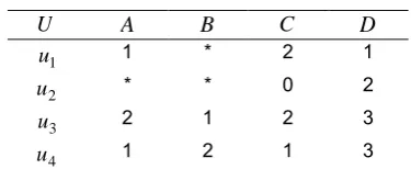
After Table 1 is reduced by A, BB and C, Table 2 is obtained.
Table 2. Reduction {A,B,C}
U A B C D
1
u 1 * 2 1
2
u * * 0 2
3
u 2 1 2 3
4
u 1 2 1 3
From another view, each object in decision table entails one classification rule, so decision table, in fact, is a set of logic rules. For instance, object 1 in Table 2 entails the rule, IF (A'1') and (C'2') THEN D'1', and object 2 entails the rule, IF (C'0') THEN D'2'.
The reduction process of decision table, virtually, is that of extracting classification rules. Rules acquired by way of reduction may be further reduced, i.e., removing those subordinate attributes irrelevant to classification. The asterisk ‘*’ in Table 2 denotes the attribute’s value isn’t important.
Reduction is the essence of RS method. It is the hotspot in machine learning and data mining and is also the theoretical basis of the proposed method.
2.2. Description of word meaning
A word has a clear meaning in a specific context, i.e., it is context that determines the sense of a word.
Suppose that the sense items set of the multi-sense word W is S{s1,s2,...,sn}. In a certain corpus, its context words
set is,
} ,..., ,
{w1 w2 wm
WordSet (1)
then corresponding to WordSet, there is a partition,
} ,..., ,
{SW1 SW2 SWn
SW (2)
satisfied
j i n j i SW SW WordSet
SWi i j
, ,, 1,..., ,
in which SWi determines si uniquely. Now we may view
i
SW as si, i.e., SWisi.
If W is in context C and its word meaning is si, we refer
the set of words in context as attributes of si and write it as
i word , where
}
,...,
,
{
i1 i2 ik iw
w
w
word
, wordiWordSet and wordi must be represented by SW , wijSWi ,i i s
Because context words are in an open set, we must go through a reduction process when sense of W is determined. Data sparseness is one problem in attribute values reduction. Some elementary categories are covered by a partition of condition attributes, but that coverage may be incomplete, that is, these categories shouldn’t be covered.
In theory, knowledge acquired by reduction of RS doesn’t lose information in corpora, but corpora are approximate representation of some information of natural language. Therefore, the amount of information in corpora is less than that of knowledge in natural language, which leads to knowledge discovering by attribute values reduction based on corpora only approximating to natural language.
2.3. Brief to IL
Instance-based learning is a machine learning method evolving from memory-based reasoning. This reasoning pattern supposes that reasoning of knowledge is more a process of similarity comparison based on experience than a process of condition-action based on conception induction. It is based on the hypothesis that the learning process is memory based.
The knowledge representation in IL is attribute logic, too. Similarity degree is computed with formula (3).
ni
i i i
x
y
W
y
x
1
)
,
(
)
,
(
(3)According to the knowledge representation system defined in section 2.1, x,yU , xi,yiV , iC ,
i x i X
f( , ) , f(Y,i)yi , where wi is the weight of attribute i which determines its importance, and (xi,yi) is
the distance of discrete attributes.
The classification based on formula (1) needs to traverse all instances in memory learning, find the instance N having nearest distance and tag the instance classified with decision attribute of N.
2.4. Natural language and instance-based
learning
The similarity reasoning mechanism of IL has 2 advantages in NLP.
Knowledge acquisition without information lost A lot of knowledge in natural language processing is difficult to represent and acquire. Learning process in memory eases this problem in some degree.
Paying more attention to outliers
The difficulty to represent natural language is there are many outliers in it. The reasoning mechanism of IL pays more attention to outliers. Reasoning of IL is more accurate than dualism, which is a reasoning theory -- if it is not A then it must be B.
3. RS and IL based knowledge acquisition
of Chinese multi-sense verbs
We use Contemporary Chinese Dictionary (CCD) and HowNet as lexicographic resources and select multi-sense verbs in both dictionaries, or else we may select the one which has only one sense as the verb’s sense.
There are 2 major modules in knowledge acquisition: original decision table generation and RS based attribute reduction.
3.1. Module of original decision table
generation
The generation of original table is shown in Figure 1.
1. For each multi-sense verb do the step ii-iv; 2. Recognizing all sentences containing the verb
in corpora;
3. Selecting manually a sense for the multi-sense verb according to the context;
4. Putting the sense and corresponding context words into table.
Figure 1. Pseudocode of decision table generation
There are 16 fields in the decision table -- wd_0, SINHN, SINXH, wd_6, wd_5, wd_4, wd_3, wd_2, wd_1, wd1, wd2, wd3, wd3, wd4, wd5, wd6, number. SINHN, SINXH are decision attributes. They are the sense of the multi-sense verb in HowNet and CCD respectively. Wd_6~wd_1, which are 6 context words previous to the multi-sense verb in the sentence, and wd1~wd6, which are 6 context words succeeding the verb, are condition attributes. Number is used to count the same instances in the corpora, that is, the number of sentences which can produce the same record in the decision table.
The major words deciding the verb sense in a sentence are nouns and there are at most 5 slots modifying the headword from different angles before a specific noun [23]. Therefore we may get the noun determining the verb sense by extracting 6 context words previous and succeeding to the multi-sense verb respectively. If the number of context words prior to or succeeding the verb is less than 6, we’ll assign a liberty value to it (them), denoting by ‘*’. The record obtained from the sample sentence is shown in Table 3.
Table 3. Description of data in decision table
SINHN SINXH wd_6 wd_5 wd_4 wd_3 wd_2 wd_1 wd_0 wd1 wd2 wd3 wd4 wd5 wd6 number
002831 418340-1 这 一 优势 更 多 地 表现 在 资源 上 但是 农业 产业化 **
Example:
虽然 c 眼下 t 这 r 一 m 优势 n 更 d 多 a 地 u 表现 v 在 p 资源 n 上 f , w 但是 c 农业 n 产业化 vn 的 u 发展 vn , w 已经 d 开始 v 将 p 资源 n 优势 n 逐步 d 转化 v 为 v 经 济 n 优势 n 。
3.2. Module of RS based attribute reduction
Knowledge is acquired by reduction of original decision table based on RS reduction.
Basic Algorithm
The algorithm includes three main procedures: PreProcess, AcquireProcess and ExceptionRule.
Preprocess
In this procedure, those conditional attributes with none of the same value are removed, because they cannot produce reduction rules.
ExceptionRule
It is used to copy instance(s) not entailed by any rule, i.e., outliers, to the table ExceptionTable.
AcquireProcess
This is fulfilled by 2 procedures. First, ProduceFromLtoS extracts rules composed by most attributes to candidate table “RuleTable” from decision table “worktable”. Second, ProduceFromStoL extracts rules from RuleTable according to the length of rules. This procedure gives priority to rules with least length, that is, if a longer rule is entailed by a shorter rule, then the longer rule is removed. Actually, ProduceFromStoL removes redundant information from RuleTable. This assures rules acquired contain least attributes yet classification is also correct.
The pseudo code can be seen in Figure 2 and Figure 3. LenofContext is the number of context words prior to or succeeding to the given multi-sense verb. It is assumed as 7 in this paper.
while not(worktable.eof) do begin
for k:=2*LenofContext to 1 do begin
If exists other record(s) having the same value as present record in any k attributes?
Yes, regard the k attributes as the conditional attributes of a rule and test if the decision table is coordination?
Yes, add this rule to candidate table RuleTable and remove all records having the same value as present record in the k attributes from worktable; end;
move to next record; end;
Figure 2. Pseudocode of ProduceFromLtoS
When ProduceFromLtoS is finished, records in worktable are outliers, which can be copied to ExceptionTable by procedure ExceitpionRule.
for i:=1 to 2*LenofContext do
while exists rule with length i and unprocessed begin
Generate a rule with length i;
Remove all rules with length greater than i and entailed by this rule;
Tag the rule with processed; end
Figure 3 Pseudocode of ProduceFromStoL
Time Complexity of the Algorithm
In an original decision table, assume the number of conditional attributes is m, the number of records is n, reduction algorithm consumes most time in ProduceFromLtoS, which shoud be executed O(2m) times and the time complexity itself is O(n2). Thus, in worst case,
the time complexity of reduction algorithm is O(2mn2). By PreProcess, some conditional attributes may be removed because they cannot play any role in reduction, thus the search scale will be reduced dramatically.
Incremental Algorithm
As seen in the previous paragraph, the complexity of computing reduction increases exponentially with the increase in scale of decision table. The introduction of a heuristic search method will help in discovering a better reduction with least conditional attributes.
When new knowledge is added to decision table, it is necessary to acquire rules by an incremental algorithm.
The idea is naïve and its correctness is obvious. It is shown in Figure 4.
1. Remove new instances covered by existed rules from new decision table;
2. Merge remaining new instances with outliers in ExceptionTable
3. Call Basic Algorithm to fulfill the acquisition of rules.
Figure 4. Incremental learning Algorithm
Short of empirical knowledge about data sparseness, we define a threshold as number of instances covered by a candidate rule, to avoid distortion of induction and errors of automatic knowledge acquisition caused by data sparseness in some degree. Only when the number of instances covered by a candidate rule is greater than or equal to , can it be selected as an eligible rule.
1. To avoid problem caused by data sparseness efficiently.
2. To filter ‘noise’. ‘Noise’ may cause outliers independent of any category and reduction based on RS attribute values may include outliers in a rule set. This will lead to such a result that the inference must comply with dualism. The threshold
canavoid including outliers in a rule set.
3. To increase time and space efficiency of machine learning. The threshold
may limit effectively theexcess inflation of the candidate rule set caused by data sparseness. Therefore, the time and space efficiency is increased.
3.3. Knowledge representation
Two kinds of knowledge are generated by reduction of decision table. One is rules covering instances greater than or equal to the given threshold . The other is instances that can’t form a rule because it covers instances less than . We use generation rules to describe these rules which have different implementing forms for the specific data.
Because rules have varied condition attributes, it is so wasteful to describe them with a table (decision table) that we build a rule file, which is a text file, to store them. The format of the text file is:
word(i).Ri.XH=Sense in XH word(i).Ri.HN=Sense in HN word(i).Ri.wd(a)=value(a) ……
word(i).Ri.wd(n)=value(n)
word(i).Ri.len=Number of words contained in the rule i The first two items are decision attributes, the last item denotes length of the rule, i.e., the number of words determining the rule, and other items are condition attributes. It means if verbword(i) and context word avalue(a)
context word bvalue(b) … then the verb sense in CCD is Sense in XH, in HowNet is Sense in HN.
We collect those instances that can’t form a rule into a table called as “ExceptionTable”. ExceptionTable has the same structure as the original table, so it appears as a decision table. Because the instances that may form a rule have been filtered out, the scale of ExceptionTable is much smaller than the original table. Data in ExceptionTable may be used as outliers in NLP.
4. Experimental Results
4.1. Rule extraction
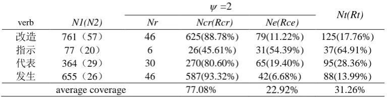
We have performed experiment with the method proposed in this paper on corpora of 5 million characters. The experiment is oriented to 4 multi-sense Chinese verbs. Because the scale of the corpora isn’t great enough, we empirically assign 2 to -- the number of instances covered in the experiment on the condition that when 1 instance is covered, it is not a law but a contingency, but when more than 1 instance are covered, it is most probably a rule. The experiment results are shown in Table 4.
Table 4. Experiment data in learning phase
=2Nt(Rt)
verb N1(N2) Nr Ncr(Rcr) Ne(Rce)
改造 761(57) 46 625(88.78%) 79(11.22%) 125(17.76%)
指示 77(20) 6 26(45.61%) 31(54.39%) 37(64.91%)
代表 364(29) 30 270(80.60%) 65(19.40%) 95(28.36%)
发生 655(26) 46 587(93.32%) 42(6.68%) 88(13.99%)
average coverage 77.08% 22.92% 31.26%
This paper using Chinese articles as the test set. So the example includes some Chinese characters. In this table, the Chinese verbs are all multi-sense words. Each word indicates different means in different conditions according the context. So the analysis of Chinese verbs is more complex. Now the English means of the multi-sense words are given as follows.
The Chinese word “改造” has three synonyms. They are “改变”, “改良” and “制造”. Their English means are “alter”, “improve” and “produce” respectively.
The Chinese word “指示” has three synonyms too. They are “指代”, “命令” and “教”. Their English means are “mean”, “order” and “teach” respectively.
The Chinese word “代表” has two synonyms. They are “指代” and “代替”. Their English means are “mean” and “replace” respectively.
And the Chinese word “发生” has two synonyms too. They are “发生” and “制造” . Their English means are “happen” and “produce” respectively.
Explanation
Rce is the corresponding coverage. Nt=Nr+Ne, and Rt, computed with formula (4), is total coverage of rules.
% 100 2 1
N N NtRt
- (4)
Coverage shows the degree of redundant information in training set reduced in the process of rule acquisition.
If there are redundant instances in training set, preserve only one instance before rule extraction. That is, redundant instances only are taken into consideration once as if they only occurred once.
Analysis
It is shown in Table 4 that in all instances experimented, on average, there is 77.08% of instance covered by rules. The highest is “发生”; its coverage is 93.32%.
The number of “rules + outliers” is 31.26% of original table averagely, so the scale of table is declined dramatically.
While the number of training instances increases, the number of rules and coverage increase accordingly.
4.2. Disambiguation
To verify the availability of acquired rules, we use them in WSD task.
Disambiguation strategy
Rule matching
Match context words of a multi-sense verb with rules in rule base. If they are matched, tag the verb with the verb sense in the rule. In matching, the priority is given to the longest rule.
Calculating average semantic distances of rules
If no rule can be matched, calculate the distance from the context words to rules with formula (5), which is the distance function between two words. Select the rule with minimum average semantic distance and tag the verb with its decision attributes.
i y and i x i x is i y or i y is i x i y is i x i y and i x i y i x between relation semantic defined no is there if 3 between distance and of hyponym of hyponym if versa vice and of hyponym immediate if between exists relation synonymy ifs
hierarchie
, 100 , 10 , 1 , 0 ) , ( (5)Actually, this is an expansion to basic rules by way of semantic classes and it is a good solution to data sparseness problem. Here, the semantic classes used are hyponymy and synonymy relation defined in HowNet.
The average semantic distance function is shown as formula (6).
n
y
x
W
y
x
n i i i iavg
(
,
)
(
,
)
/
1
Calculating the distance to outliers
If the minimum distance to rules is unacceptable, for example, the minimum distance being 100, calculate the semantic distance to outliers. Select the outlier with minimum distance and tag the multi-sense verb with its decision attribute. When computing the distance to an outlier, distance function between two words is formula (7).
i i i i i iy
x
y
x
y
x
,
1
,
0
)
,
(
(7)Experimental results
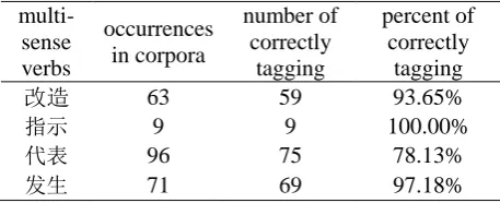
We have validated the strategy above by experiments. The percentage of correct disambiguation in close test is 100%. When experimented on open corpora of 500 thousand characters that came from journal articles, we got 92%. The detailed results of decision are shown in Table 5.
Table 5. Decision table
multi-sense verbs occurrences in corpora number of correctly tagging percent of correctly tagging
改造 63 59 93.65%
指示 9 9 100.00%
代表 96 75 78.13%
发生 71 69 97.18%
The English means of the Chinese characters are explicated in section 4.1.
5. Conclusion
We put forward and implemented an acquisition method of word senses knowledge of Chinese verbs based on RS theory and IL. We proposed conception of threshold, i.e., instances covered by a rule, to solve data sparseness problem, filter instances not governed by rules and improve time and space efficiency in machine learning of NLP. There are two problems which must be pointed out and dug deeper into in future.
representation itself may bring about data sparseness problem. So knowledge representation should be studied further.
2. Without enough corpora, rules acquired depend on training corpora to some degree.
Acknowledgements
This work was partly supported by National Natural Science Foundation of China (61202290, 61370173), Zhejiang Provincial Natural Science Foundation of China (LY12F02012), Zhejiang Province Public Technology Applied Research Project (2011C23132) and Key Innovative Research Team of Huzhou: Internet of Things - Technology & Application (2012KC04).
References
[1] H Wang, Y Zhang, J Cao, Effective collaboration with information sharing in virtual universities[J], IEEE Transactions on Knowledge and Data Engineering, 21 (6): 840-853.
[2] H Wang, J Cao, Y Zhang, A flexible payment scheme and its role-based access control[J], IEEE Transactions on Knowledge and Data Engineering, 17 (3): 425-436. [3] T.K. Das, D.P. Acharjya. A decision making model using
soft set and rough set on fuzzy approximation spaces[J]. International Journal of Intelligent Systems Technologies and Applications, 2014, 13(3): 170-186.
[4] Ouyang Yuping, Shieh Howming, Tzeng Gwohshiung, Yen Leon and Chan Chienchung. Combined rough sets with flow graph and formal concept analysis for business aviation decision-making[J]. Journal of Intelligent Information Systems, 2009, (11): 1-20.
[5] Tiecheng Bai, Hongbing Meng, Jianghe Yao. A forecasting method of forest pests based on the rough set and PSO-BP neural network[J]. Neural Computing & Applications, 2014, 25(7-8): 1699-1707.
[6] Wu Zhaoqi, Fu Chun, Zhang Chunming, Jiang Shaofei. A Revised Counter-Propagation Network Model Integrating Rough Set for Structural Damage Detection[J]. International Journal of Distributed Sensor Networks, 2013. [7] Jun Wang, Jiaxu Peng, Ou Liu. A classification approach
for less popular webpages based on latent semantic analysis and rough set model[J]. Expert Systems with Applications, 2015, 42(1): 642-648.
[8] Huang Zhengxing, Lu Xudong and Duan Huilong. Context-aware recommendation using rough set model and collaborative filtering[J]. Artificial Intelligence Review, 2010, (11): 1-15.
[9] Jhieh-Yu Shyng, How-Ming Shieh, Gwo-Hshiung Tzeng, Shu-Huei Hsieh. Using FSBT technique with Rough Set Theory for personal investment portfolio analysis[J]. European Journal of Operational Research, 2009.
[10] H Wang, Y Zhang, J Cao, Formal authorisation allocation approaches for permission-role assignments using relational algebra operations[C]. Proceedings of the 14th Australasian database conference, 2003, 17: 125-133. [11] Z. Pawlak and A. Skowron. Rudiments of rough sets[J].
Information Sciences, 2007, 177 (1): 3-27.
[12] Z. Pawlak and A. Skowron. Rough sets: Some extensions[J]. Information Sciences, 2007, 177 (1): 28-40. [13] A.R. Hedar, J. Wang and M. Fukushima. Tabu search for
attribute reduction in rough set theory[J]. Soft Computing -A Fusion of Foundations, Methodologies and -Applications, 2008, 12 (9): 909-918.
[14] Xianyong Zhang, Duoqian Miao. Region-based quantitative and hierarchical attribute reduction in the two-category decision theoretic rough set model[J]. Knowledge-Based Systems, 2014, 71(000):146-161. [15] Majdi Mafarja, Salwani Abdullah. A fuzzy
record-to-record travel algorithm for solving rough set attribute reduction[J]. International Journal of Systems Science, 2015, 46(3): 503-512.
[16] Liu Yong, Huang Wenliang, Jiang Yunliang, and Zeng Zhiyong. Quick attribute reduct algorithm for neighborhood rough set model[J]. Information Sciences, 2014, 271: 65-81.
[17] Li Li, Lu Sun, Jiayang Wang. Multi-source Knowledge Acquisition Model based on Rough Set[J]. Information Technology Journal, 2014, 13(7): 1386-1390.
[18] Wenhao Shu, Hong Shen. Incremental feature selection based on rough set in dynamic incomplete data[J]. Pattern Recognition, 2014, 47(12): 3890-3906.
[19] S. Varges and C. Mellish. Instance-based natural language generation[J]. Natural Language Engineering, 2010, 16 (3): 309-346.
[20] R. Navigli. Word sense disambiguation: A survey[J]. ACM Computing Surveys,2009, 41(2): 1-69.
[21] Gao Hongmin, Zhou Hui, Xu Lizhong, etc. Classification of hyperspectral remote sensing images based on simulated annealing genetic algorithm and multiple instance learning[J]. Journal of Central South University of Technology, 2014, 21: 262-271.
[22] Sotiris Kotsiantis. Increasing the accuracy of incremental naive bayes classifier using instance based learning [J]. International Journal of Control, Automation and Systems, 2013, 11(1): 159-166.