University of Pennsylvania
ScholarlyCommons
Publicly Accessible Penn Dissertations
2018
Resilient Submodular Maximization For Control
And Sensing
Vasileios Tzoumas
University of Pennsylvania, [email protected]
Follow this and additional works at:
https://repository.upenn.edu/edissertations
Part of the
Electrical and Electronics Commons, and the
Robotics Commons
This paper is posted at ScholarlyCommons.https://repository.upenn.edu/edissertations/3029
Recommended Citation
Tzoumas, Vasileios, "Resilient Submodular Maximization For Control And Sensing" (2018).Publicly Accessible Penn Dissertations. 3029.
Resilient Submodular Maximization For Control And Sensing
Abstract
Fundamental applications in control, sensing, and robotics, motivate the design of systems by selecting system elements, such as actuators or sensors, subject to constraints that require the elements not only to be a few in number, but also, to satisfy heterogeneity or interdependency constraints (called matroid constraints). For example, consider the scenarios:
- (Control) Actuator placement: In a power grid, how should we place a few generators both to guarantee its stabilization with minimal control effort, and to satisfy interdependency constraints where the power grid must be controllable from the generators?
- (Sensing) Sensor placement: In medical brain-wearable devices, how should we place a few sensors to ensure smoothing estimation capabilities?
- (Robotics) Sensor scheduling: At a team of mobile robots, which few on-board sensors should we activate at each robot ---subject to heterogeneity constraints on the number of sensors that each robot can activate at each time--- so both to maximize the robots' battery life, and to ensure the robots' capability to complete a formation control task?
In the first part of this thesis we motivate the above design problems, and propose the first algorithms to address them. In particular, although traditional approaches to matroid-constrained maximization have met great success in machine learning and facility location, they are unable to meet the aforementioned problem of actuator placement. In addition, although traditional approaches to sensor selection enable Kalman filtering capabilities, they do not enable smoothing or formation control capabilities, as required in the above problems of sensor placement and scheduling. Therefore, in the first part of the thesis we provide the first algorithms, and prove they achieve the following characteristics: provable approximation performance: the algorithms guarantee a solution close to the optimal; minimal running time: the algorithms terminate with the same running time as state-of-the-art algorithms for matroid-constrained maximization; adaptiveness: where applicable, at each time step the algorithms select system elements based on both the history of selections. We achieve the above ends by taking advantage of a submodular structure of in all aforementioned problems ---submodularity is a diminishing property for set functions, parallel to convexity for continuous functions.
But in failure-prone and adversarial environments, sensors and actuators can fail; sensors and actuators can get attacked. Thence, the traditional design paradigms over matroid-constraints become insufficient, and in contrast, resilient designs against attacks or failures become important. However, no approximation algorithms are known for their solution; relevantly, the problem of resilient maximization over matroid constraints is NP-hard.
In the second part of this thesis we motivate the general problem of resilient maximization over matroid constraints, and propose the first algorithms to address it, to protect that way any design over matroid constraints, not only within the boundaries of control, sensing, and robotics, but also within machine learning, facility location, and matroid-constrained optimization in general.
In particular, in the second part of this thesis we provide the first algorithms, and prove they achieve the following characteristics: resiliency: the algorithms are valid for any number of attacks or failures;
algorithms guarantee for any submodular or merely monotone function a solution close to the optimal; minimal running time: the algorithms terminate with the same running time as state-of-the-art algorithms for matroid-constrained maximization. We bound the performance of our algorithms by using notions of curvature for monotone (not necessarily submodular) set functions, which are established in the literature of submodular maximization.
In the third and final part of this thesis we apply our tools for resilient maximization in robotics, and in particular, to the problem of active information gathering with mobile robots. This problem calls for the motion-design of a team of mobile robots so to enable the effective information gathering about a process of interest, to support, e.g., critical missions such as hazardous environmental monitoring, and search and rescue. Therefore, in the third part of this thesis we aim to protect such multi-robot information gathering tasks against attacks or failures that can result to the withdrawal of robots from the task. We conduct both numerical and hardware experiments in multi-robot multi-target tracking scenarios, and exemplify the benefits, as well as, the performance of our approach.
Degree Type Dissertation
Degree Name
Doctor of Philosophy (PhD)
Graduate Group
Electrical & Systems Engineering
First Advisor George J. Pappas
Second Advisor Ali Jadbabaie
Subject Categories
RESILIENT SUBMODULAR MAXIMIZATION FOR CONTROL AND SENSING
Vasileios Tzoumas
A DISSERTATION
in
Electrical and Systems Engineering
Presented to the Faculties of the University of Pennsylvania
in
Partial Fulllment of the Requirements for the
Degree of Doctor of Philosophy
2018
Dissertation Supervisor
George J. Pappas, Professor of Electrical and Systems Engineering (UPenn)
Dissertation Co-Supervisor
Ali Jadbabaie, Professor of Engineering, Institute for Data, Systems and Society (MIT)
Graduate Group Chairperson
Alejandro Ribeiro, Associate Professor of Electrical and Systems Engineering (UPenn)
Dissertation Committee
Rakesh Vohra, Professor of Economics and of Electrical and Systems Engineering (UPenn)
Hamed Hassani, Assistant Professor of Electrical and Systems Engineering (UPenn)
RESILIENT SUBMODULAR MAXIMIZATION FOR CONTROL AND SENSING
c
COPYRIGHT
2018
ABSTRACT
RESILIENT SUBMODULAR MAXIMIZATION FOR CONTROL AND SENSING
Vasileios Tzoumas George J. Pappas
Ali Jadbabaie
Fundamental applications in control, sensing, and robotics, motivate the design of systems by selecting system elements, such as actuators or sensors, subject to constraints that require the elements not only to be a few in number, but also, to satisfy heterogeneity or interde-pendency constraints (called matroid constraints). For example, consider the scenarios:
• (Control) Actuator placement: In a power grid, how should we place a few generators
both to guarantee its stabilization with minimal control eort, and to satisfy interde-pendency constraints where the power grid must be controllable from the generators?
• (Sensing) Sensor placement: In medical brain-wearable devices, how should we place
a few sensors to ensure smoothing estimation capabilities?
• (Robotics) Sensor scheduling: At a team of mobile robots, which few on-board sensors
should we activate at each robot subject to heterogeneity constraints on the number of sensors that each robot can activate at each time so both to maximize the robots' battery life, and to ensure the robots' capability to complete a formation control task?
In the rst part of this thesis we motivate the above design problems, and propose the rst algorithms to address them. In particular, although traditional approaches to matroid-constrained maximization have met great success in machine learning and facility location, they are unable to meet the aforementioned problem of actuator placement. In addition, although traditional approaches to sensor selection enable Kalman ltering capabilities, they do not enable smoothing or formation control capabilities, as required in the above problems of sensor placement and scheduling. Therefore, in the rst part of the thesis we provide the rst algorithms, and prove they achieve the following characteristics: prov-able approximation performance: the algorithms guarantee a solution close to the optimal; minimal running time: the algorithms terminate with the same running time as state-of-the-art algorithms for matroid-constrained maximization; adaptiveness: where applicable, at each time step the algorithms select system elements based on both the history of se-lections. We achieve the above ends by taking advantage of a submodular structure of in all aforementioned problems submodularity is a diminishing property for set functions, parallel to convexity for continuous functions.
In the second part of this thesis we motivate the general problem of resilient maximization over matroid constraints, and propose the rst algorithms to address it, to protect that way any design over matroid constraints, not only within the boundaries of control, sensing, and robotics, but also within machine learning, facility location, and matroid-constrained optimization in general. In particular, in the second part of this thesis we provide the rst algorithms, and prove they achieve the following characteristics: resiliency: the algorithms are valid for any number of attacks or failures; adaptiveness: where applicable, at each time step the algorithms select system elements based on both the history of selections, and on the history of attacks or failures; provable approximation guarantees: the algorithms guarantee for any submodular or merely monotone function a solution close to the optimal; minimal running time: the algorithms terminate with the same running time as state-of-the-art algorithms for matroid-constrained maximization. We bound the performance of our algorithms by using notions of curvature for monotone (not necessarily submodular) set functions, which are established in the literature of submodular maximization.
TABLE OF CONTENTS
ABSTRACT . . . ii
LIST OF ILLUSTRATIONS . . . ix
CHAPTER 1 : INTRODUCTION . . . 1
1.1 Motivation of submodular maximization in control, sensing, and robotics . . . 1
1.2 State-of-the-art approaches for submodular maximization . . . 2
1.3 Need for novel approaches of submodular maximization in control . . . 3
1.4 Need for novel approaches of submodular maximization in sensing and robotics 4 1.5 Need for resilient submodular maximization . . . 4
1.6 Thesis goal and approach . . . 6
1.7 Thesis contributions, and organization . . . 8
I CONTRIBUTIONS TO SUBMODULAR MAXIMIZATION IN ACTUATION DESIGN 12 CHAPTER 2 : Minimal Reachability is Hard to Approximate . . . 13
2.1 Introduction . . . 13
2.2 Minimal Reachability Problem . . . 15
2.3 Non-supermodularity of distance from point to subspace . . . 16
2.4 Inapproximability of Minimal Reachability Problem . . . 18
2.5 Proof of Inapproximability of Minimal Reachability . . . 19
2.6 Concluding Remarks & Future Work . . . 24
CHAPTER 3 : Minimal Actuator Placement with Bounds on Control Eort . . . 26
3.1 Introduction . . . 26
3.2 Problem Formulation . . . 28
3.3 Minimal Actuator Sets with Constrained Control Eort . . . 33
3.4 Minimum Energy Control by a Cardinality-Constrained Actuator Set . . . 39
3.5 Concluding Remarks & Future Work . . . 42
3.6 Appendix: Computational Complexity . . . 42
II CONTRIBUTIONS TO SUBMODULAR MAXIMIZATION IN SENSING DESIGN 45 CHAPTER 4 : Sensor Placement for Optimal Kalman Filtering: Fundamental Lim-its, Submodularity, and Algorithms . . . 46
4.1 Introduction . . . 46
4.2 Problem Formulation . . . 48
4.4 Submodularity in Optimal Sensor Placement . . . 53
4.5 Algorithms for Optimal Sensor Placement . . . 54
4.6 Concluding Remarks & Future Work . . . 56
4.7 Appendix: Proof of Results . . . 56
CHAPTER 5 : Near-optimal sensor scheduling for batch state estimation: Complex-ity, algorithms, and limits . . . 60
5.1 Introduction . . . 60
5.2 Problem Formulation . . . 63
5.3 Main Results . . . 65
5.4 Concluding Remarks & Future Work . . . 71
5.5 Appendix: Proof of Results . . . 71
CHAPTER 6 : Selecting sensors in biological fractional-order systems . . . 75
6.1 Introduction . . . 75
6.2 Problem Statement . . . 78
6.3 Sensor Placement for DTFOS . . . 83
6.4 EEG Sensor Placement . . . 86
6.5 Concluding Remarks & Future Work . . . 92
6.6 Appendix: Proof of the Results . . . 93
CHAPTER 7 : Scheduling Nonlinear Sensors for Stochastic Process Estimation . . . 99
7.1 Introduction . . . 99
7.2 Problem Formulation . . . 102
7.3 Main Results . . . 103
7.4 Conclusion Remarks & Future Work . . . 107
7.5 Appendix: Proof of Results . . . 107
CHAPTER 8 : LQG Control and Sensing Co-design . . . 112
8.1 Introduction . . . 112
8.2 LQG Control and Sensing Co-design: Problem Statement . . . 115
8.3 Co-design Principles and Ecient Algorithms . . . 119
8.4 Performance guarantees for LQG Co-Design . . . 124
8.5 Numerical Experiments . . . 132
8.6 Concluding Remarks & Future Work . . . 136
8.7 Appendix: Proof of Results . . . 137
III RESILIENT SUBMODULAR MAXIMIZATION 160 CHAPTER 9 : Resilient Non-Submodular Maximization over Matroid Constraints . 161 9.1 Introduction . . . 161
9.2 Resilient Non-Submodular Maximization over Matroid Constraints . . . 164
9.3 Algorithm for Problem 4 . . . 167
9.4 Performance Guarantees for Algorithm 19 . . . 169
9.6 Concluding Remarks & Future Work . . . 176
9.7 Appendix: Proof of Results . . . 177
CHAPTER 10 : Resilient (Non-)Submodular Sequential Maximization . . . 189
10.1 Introduction . . . 189
10.2 Resilient Monotone Sequential Maximization . . . 192
10.3 Adaptive Algorithm for Problem 5 . . . 193
10.4 Performance Guarantees for Algorithm 20 . . . 195
10.5 Numerical Experiments . . . 199
10.6 Concluding Remarks & Future Work . . . 201
10.7 Appendix: Proof of Results . . . 202
IV CONTRIBUTIONS TO RESILIENT SUBMODULAR MAXI-MIZATION IN ROBOTICS 213 CHAPTER 11 : Resilient Active Information Gathering with Mobile Robots . . . 214
11.1 Introduction . . . 214
11.2 Problem Statement . . . 216
11.3 Algorithm for Resilient Active Information gathering . . . 218
11.4 Performance Guarantees . . . 220
11.5 Application: Multi-target tracking with mobile robots . . . 224
11.6 Concluding Remarks & Future Work . . . 228
11.7 Appendix: Proof of Results . . . 230
LIST OF ILLUSTRATIONS
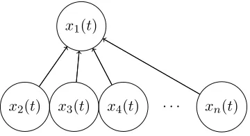
FIGURE 1 : Graphical representation of the linear system x˙1(t) = Pnj=2xj(t),
˙
xi(t) = 0, i = 2, . . . , n; each node represents an entry of the sys-tem's state (x1(t), x2(t), . . . , xn(t)), where t represents time; the
edges denote that the evolution in time ofx1depends on(x2, x3, . . . ,
xn). . . 14
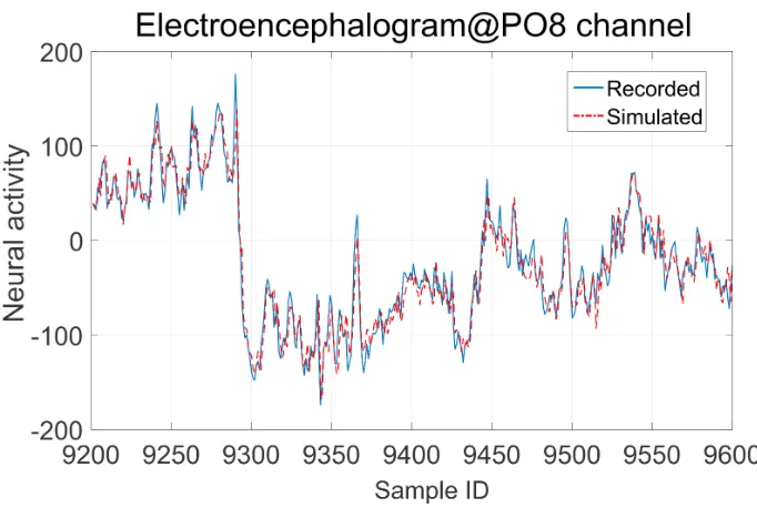
FIGURE 2 : EEG data recorded and the simulated using DTFOS at the EEG channel
PO8. . . 87
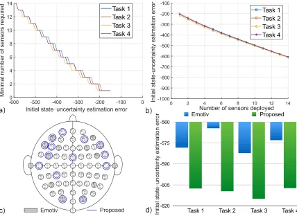
FIGURE 3 : (a) Minimal sensor placement to achieve a prescribed initial
state-uncertainty estimation errors. (b) initial state-state-uncertainty log det
errors achieved given dierent sensor budgets. (c) The 64-channel geodesic sensor distribution for measurement of EEG, where the sensors in gray represent those of the Emotiv EPOC and the ones
in red are those returned by Algorithm 12 when solving (P2) (that
relieved to be the same for all 4 tasks), given the identied DT-FOS and a deployment budget of 14 sensors. (d) initial
state-uncertaintylog detestimation errors associated with the highlighted
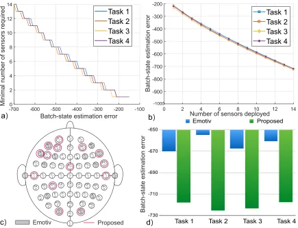
sensor placements in (c). . . 88 FIGURE 4 : (a) Minimal sensor placement to achieve a prescribed batch-state
estimation errors. (b) batch-statelog deterrors achieved given
dif-ferent sensor budgets. (c) The 64-channel geodesic sensor distribu-tion for measurement of EEG, where the sensors in gray represent those of the Emotiv EPOC and the ones in red are those returned
by Algorithm 12 when solving (P4) (that relieved to be the same for
all 4 tasks), given the identied DTFOS and a deployment budget
of 14 sensors. (d) batch-statelog det estimation errors associated
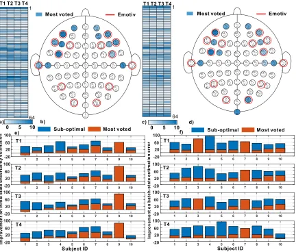
with the highlighted sensor placements in (c). . . 90 FIGURE 5 : (a-b) The 64-channel geodesic sensor distribution over 10 subjects
under Task 1-4 and the most voted deployment given a 14-sensor budget by minimizing (a) the initial state-uncertainty estimation error and (b) batch-state estimation error. (c-d) The improvement on (c) initial state-uncertainty estimation error and (d) batch-state estimation error when (i) the sub-optimal 14-sensor deployment re-turned by Algorithm 2 individually (blue bar) and (ii) the most voted 14-sensor deployment by 10 subjects (red bar) are considered. 91
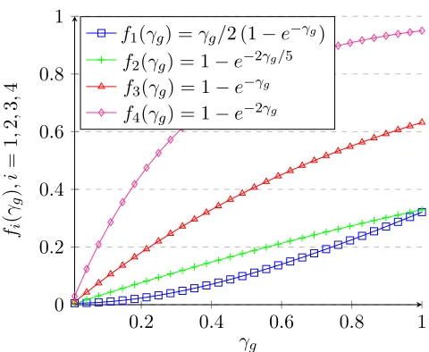
FIGURE 6 : Plot of fi(γg) (i = 1,2,3,4) versus supermodularity ratio γg of a
monotone supermodular functiong. By Denition 29 of
supermod-ularity ratio,γg takes values between0and1. Asγg increases from
0to 1 then: f1(γg) increases from0 to 1/2(1−e−1)'0.32;f3(γg)
increases from 0 to 1−e−2/5 ' 0.32; f2(γg) increases from 0 to
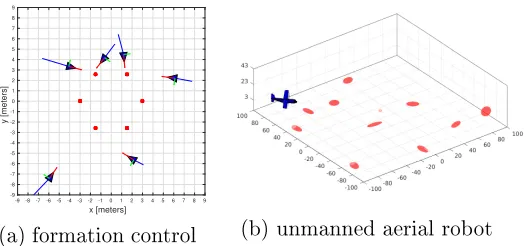
FIGURE 7 : Examples of applications of the proposed sensing-constrained LQG-control framework: (a) sensing-constrained formation LQG-control and (b) resource-constrained robot navigation. . . 133
FIGURE 8 : LQGcost for increasing (a)-(b) control horizon T, (c)-(d) number
of selected sensorsk, and (e)-(f) number of agents n. Statistics are
reported for the homogeneous formation control setup (left column), and the heterogeneous setup (right column). Results are averaged over 100 Monte Carlo runs. . . 135
FIGURE 9 : LQGcost for increasing (a) control horizon T, and (b) number of
selected sensors k. Statistics are reported for the heterogeneous
setup. Results are averaged over 100 Monte Carlo runs. . . 136
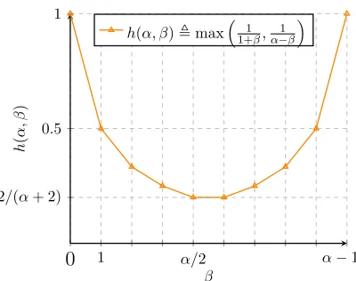
FIGURE 10 : Given a natural numberα, plot ofh(α, β)versusβ. Given a niteα, then
h(α, β)is always non-zero, with minimum value2/(α+ 2), and maximum
value1. . . 172
FIGURE 11 : Plot ofg(κf)versus curvature κf of a monotone submodular
func-tionf. By denition, the curvatureκf of a monotone submodular
functionf takes values between 0and 1. g(κf)increases from 0to
1asκf decreases from1 to 0. . . 173
FIGURE 12 : LQG cost for increasing number of sensor selectionsα(from 2 up to 12
with step1), and for4 values ofβ (number of sensor failures among the αselected sensors); in particular, the value of β varies across the
sub-gures as follows: β= 1 in sub-gure (a);β = 4in sub-gure (b);β = 7
in sub-gure (c); andβ = 10in sub-gure (d). . . 177
FIGURE 13 : Venn diagram, where the sets A1,A2,B?1,B2? are as follows: per
Algo-rithm 19,A1 andA2are such thatA=A1∪ A2. Due to their
construc-tion, it holdsA1∩A2=∅. Next,B1?andB2?are such thatB?1=B?(A)∩A1,
andB?
2 =B?(A)∩ A2; therefore,B1?∩ B2?=∅ andB?(A) = (B1?∪ B?2). . . 186
FIGURE 14 : LQG cost for increasing time, where across all sub-gures (a)-(d) it is
α= 11(number of active sensors per time step). The value ofβ(number
of sensor failures at each time step among the α active sensors) varies
across the sub-gures. . . 201
FIGURE 15 : Venn diagram, where the setsSt,1,St,2,B?
t,1,B?t,2 are as follows: per
Algorithm 20, St,1 and St,2 are such that At = St,1 ∪ St,2. In
addition, due to their construction, it holdsSt,1∩St,2 =∅. Next,Bt,?1
andB?
t,2 are such thatBt,?1 =B?(A1:T)∩ St,1, andB2?=B?(A1:T)∩ St,2; therefore, it is B?
t,1∩ Bt,?2 =∅ and B?(A1:T) = (B?1,1 ∪ B1?,2)∪
· · · ∪(B?
T ,1∪ B?T ,2). . . 210
FIGURE 16 : Simulation environment depicting ve robots. The jammed robot is
FIGURE 17 : The gures depict the average entropy and position RMSE (root mean square error) per target, averaged over the robots. Figs. (a-b) were obtained from a simulation with 10 robots, 10 targets, with 2 jamming attacks. Figs. (c-d) have the same conguration but up to 6 jamming attacks. The blue colors correspond to the non-resilient algorithm, and the red colors correspond to the resilient algorithm. The shaded regions are the spread between the minimum and maximum values of the infor-mation measure, and the solid lines are the mean value. The plots are the aggregate of ten trials, each executed over 500 time-steps. . . 226
FIGURE 18 : The experimental setup with two quad-rotors equipped with Qualcomm
FlightTM, and two Scarabs as ground targets. . . . 228
FIGURE 19 : The plot in (a) depicts the experimental robot trajectories in the
non-resilient algorithm. The gure in (b) depicts the non-resilient algorithm. The targets are in green. . . 229
FIGURE 20 : Venn diagram, where the setLis the robot set dened in step 2 of
Algo-rithm 22, and the setA?
1 and the setA?2 are such thatA?1=A?∩ L, and A?
2=A?∩(V \ L)(observe that these denitions implyA?1∩ A?2=∅and A?=A?
CHAPTER 1 : INTRODUCTION
1.1. Motivation of submodular maximization in control, sensing, and robotics
Researchers in control, sensing, and robotics envision the design of critical infrastructures and autonomous systems in applications such as:
• (Control) Power-grid stabilization: Deploy new-technology HVDC generators in power
grids to guarantee their stabilization. [1]
• (Sensing) Search and rescue: Deploy mobile robots to localize people trapped in
burn-ing buildburn-ings. [2]
• (Robotics) Multi-target coverage: Deploy aerial micro-robots to monitor targets that
move in a cluttered urban environment. [3]
In particular, all the aforementioned applications motivate fundamental set function opti-mization problems such as:
• (Control) Actuator placement: In a power grid, how should we place a few generators
both to guarantee its stabilization, and to satisfy global-interdependency constraints where the power grid must be controllable from the generators? [4]
• (Sensing) Sensor scheduling: At a team of mobile robots, which few on-board sensors
should we activate at each robot subject to heterogeneity constraints on the number of sensors each robot can activate so both to maximize the robots' battery life, and to ensure the robots' capability to complete a formation control task? [5]
• (Robotics) Motion planning: At a team of aerial robots, how should we select the
robots' motions to maximize the team's capability for tracking targets moving in ur-ban environments, subject to heterogeneity constraints where each robot has dierent motion capabilities? [6]
Specically, all the above applications motivate the design of systems by selecting system elements, such as actuators, sensors, or movements, subject to complex design constraints that require the system elements not only to be a few in number, but also to possibly satisfy heterogeneity or global-interdependency constraints. Other general fundamental problems that involve such complex design constraints are:
• (Control) Sparse actuation design for state reachability or low-control eort [4], or
merely for controllability [7] or structural controllability [8]; and synchronization in complex networks for tasks of motion coordination [9].
• (Sensing) Sparse sensing design for optimal Kalman ltering [5, 10].
• (Robotics) Task allocation in collaborative multi-robot systems for surveillance in
In more detail, all the aforementioned problems and applications require the solution to an optimization problem of the form:
max
A⊆V,A∈I f(A), (1.1)
where the setV represent a set of available elements to choose from; the setI represents the
collection of complex design constraints called matroids [12] that enforce heterogeneity
or global-interdependency across the elements in A; and the objective function f is
non-decreasing and (possibly) submodular; submodularity is a diminishing returns property. For
example, I may constrain the cardinality of each feasible set in the problem in eq. (1.1),
e.g., when I = {A :A ⊆ V,|A| ≤ α}, given some positive integer α; an interpretation of
the number α is that it captures a resource constraint, such as a limited battery for sensor
activation, which limits the number of elements one can select in A (under the implicit
assumption that all the elements in V consume the same amount of the limited resource).
In some cases, however, dierent elements may consume dierent amounts of the limited resource; for example, dierent sensors may have dierent battery consumption. In such
heterogeneity scenarios, I may constrain the cost of each feasible set in the problem in
eq. (1.1), e.g., by beingI ={A :A ⊆ V, c(A)≤b}, given some cost function c(A) over all
the possible subsets A ⊆ V, and given some budget constraintb; that is, the cost function c
captures the heterogeneity in the cost of each element in V. More generally, I may also
enforce heterogeneity to the elements inAby partitioning the elements inV, and permitting
the selection of only a few elements from each partition, e.g., whenV =V1 ∪ · · · ∪ Vn and
I ={A:A ⊆ V, ci(A ∩ Vi)≤bi, for alli= 1, . . . , n}, given a positive integer n, a partition
V1, . . . ,Vn of V, cost functions c1, . . . , cn, and budget constraints b1, . . . , bn. In particular,
we may give two interpretations of the heterogeneity introduced by the setsV1, . . . ,Vn: the
rst interpretation considers that the sets V1, . . . ,Vn correspond to the available elements
across n dierent types (buckets) of elements, and correspondingly, the budgets b1, . . . , bn
constrain the total cost of the elements one can use from each type1, . . . , n; and the second
interpretation considers that the setsV1, . . . ,Vncorrespond to the available elements across
ndierent times, and correspondingly, the budget constraints b1, . . . , bn constrain the total
cost of the elements one can use at each time 1, . . . , n. Finally, in other complex design
scenarios, that call for global-interdependency among the selected elements,I may require
the elements inA to form, e.g., a spanning tree on a graph associated toV, such as in the
aforementioned scenario of leader selection for structural controllability [8].
1.2. State-of-the-art approaches for submodular maximization
Overall, the optimization problem in eq. (1.1) is combinatorial, and, in particular, it is NP-hard [13]; notwithstanding, greedy-like algorithms have been proposed for its solution [12, 14], such as the greedy presented in Algorithm 1. Specically, Algorithm 1 builds sequentially
an approximate solution for the problem in eq. (1.1), by starting with an empty setA(line 1
of Algorithm 1), and then by adding inAone element at a time (lines 2-8 of Algorithm 1);
in particular, any element that achieves the highest value off(A ∪ {y}) among the elements
y∈ V that not chosen so far (line 5 of Algorithm 1) and for which the feasibility constraint
A ∪ {y} ∈ I is satised (lines 4 of Algorithm 1). Similarly, the rest of the state-of-the-art
Algorithm 1 Greedy algorithm for problem in eq. (1.1) [12]. Input: Per problem in eq. (1.1), Algorithm 19 receives the inputs:
• a matroid(V,I);
• a non-decreasing set functionf : 2V 7→R.
Output: SetA.
1: A ← ∅; R ← ∅;
2: whileR 6=V do
3: x∈arg maxy∈V\(A∪R)f(A ∪ {y});
4: if A ∪ {x} ∈ I then
5: A ← A ∪ {x};
6: end if
7: R ← R ∪ {x};
8: end while
steps to the ones in Algorithm 1, and dier only on how they choose which element to add
inA(i.e., they replace the criterion in line 3 of Algorithm 1 with some other).
Notably, the algorithms in [12, 14] are proved to be near-optimal for several instances of the optimization problem in eq. (1.1) [13, 14, 15], and are commonly used in, e.g., statistics, such as, in machine learning [16], and optimization, such as, in facility location [17].
1.3. Need for novel approaches of submodular maximization in control
However, the algorithms in [12, 14], cannot address with provable approximation perfor-mance the fundamental control problems of actuator selection discussed above, such as the ones in [4]. In particular, consider the fundamental problem of actuator placement for low control eort in [4], where the objective is to place a few actuators in a dynamical system to minimize the average control eort one needs to drive the system in the state space. In this case, the algorithms in [12, 14] do not exhibit the near-optimal approximation proved in [12, 15], even for average control-eort metrics (which are instances of the objective
func-tionf in eq. (1.1)) that are non-decreasing and submodular. To reveal the reason, we next
discuss in more detail when a system can be controlled with low eort from an actuator set, and then discuss how the algorithms in [12, 14] may become insucient in this context: specically, the control-eort one needs to drive a system in the state space is innite if the system is not controllable from the set of placed actuators, i.e., if there exists at least one system state that is not reachable with a nite amount of control eort from the set of placed actuators. In particular, for a system to be controllable typically more than one actuators is needed [18]. Hence, given a system, and any set of placed actuators of low enough
cardi-nality, then any metricf that captures the average control eort needed to drive the system
in the state space [19] is innity (has innite value). The latter conclusion is sucient to reveal why the algorithms in [12, 14] may fail to provide a near-optimal actuator selection for low-eort control: by focusing without loss of generality only on Algorithm 1, recall that Algorithm 1 builds an approximate solution to the optimization problem in eq. (1.1)
greedily, by starting with an empty set A, and then by adding elements in A one-by-one,
add; however, since the control eort metrics are innity insofar only a few actuators have
been added in A, Algorithm 1 cannot dierentiate among them, and as a result, it picks
randomly the element to add inA. The complication of this fact is that even though all the
elements nally picked in A aect the average control eort, a part of A has been picked
randomly, instead for minimizing the average control eort.
In sum, we have exemplied the necessity for novel tools of submodular maximization in control, by presenting the above complications in applying the state-of-the-art algorithms in [12, 14] to the fundamental problem of actuator placement for low control eort.
1.4. Need for novel approaches of submodular maximization in sensing and robotics
Traditional designs in sensing focus on selecting sensors in critical infrastructures, such as in networks of satellites, or in power-grids, with the objective to enable state estimation via Kalman ltering in the presence of resource constraints, such as of limited bandwidth for simultaneous satellite sensor communication [20], or of limited monetary budget for phasor-measurement-unit (PMU) placement in power grids [4].
However, recent advances in the miniaturization of sensors and robots trigger the vision of using swarms of mobile robots to support missions of search and rescue, and of safety and security [2], which all suggest a shift of focus in the sensor selection process beyond Kalman ltering: in particular, a shift from sensor selection for merely state estimation (Kalman ltering) to sensor selection for autonomous navigation. For example, for a swarm of robots to participate in missions of search and rescue in burning buildings, where each robot in the swarm can operate only a subset of its sensors due to limited battery, the primary goal of the sensor selection process is to enable the swarm's capability for autonomous navigation, instead of its capability for only localization (state estimation); that is, such missions of autonomous navigation exemplify the need for navigation-aware sensor selection emerges, instead of merely localization-aware sensor selection.
At the same time, emergent medical applications require the design of multi-sensor devices, such as of brain wearables, that enable smoothing estimation (trajectory estimation), instead of Kalman ltering (state estimation); see [21] and the references therein. Similarly, research in robotics weigh also on smoothing estimation to enable exploration missions in unknown environments by the means of simultaneous localization and mapping (SLAM) [22].
In sum, novel sensor selection schemes of submodular maximization are necessitated, that go beyond Kalman ltering to enable a variety of critical applications such as medical ap-plications of brain wearables, and autonomous navigation apap-plications of swarms of robots.
1.5. Need for resilient submodular maximization
denial-of-service attacks and failures, either in an o-line fashion (before any attack or failure happens) or in an on-line fashion (while any attacks or failures happen).
Evidently, which of the two options is appropriate o-line or on-line resilient design depends on the context of the design in hand. For example, o-line protection of designs becomes important in critical infrastructures, such as in power grids, where the design happens once, does not change in time, and needs to withstand future attacks or failures [1, 25]. In contrast, on-line protection of designs becomes important in critical tasks where the design requirements may evolve in time, such as in sensor scheduling for autonomous navigation in search and rescue, where, specically, dierent sensors are activated at each time step, and as a result, dierent sensors may fail or get attacked at each time step.
We discuss in more detail the two options of o-line and on-line resilient design below.
1.5.1. O-line resilient submodular maximization
An option for an o-line resilient re-formulation of the problem in eq. (1.1) is the following:
max
A⊆V,A∈I B⊆Amin,B∈I0 f(A \ B). (1.2)
where the set I0 represents the collection of possible set-removalsB attacks or failures
from A, each of some specied cardinality. Hence, the problem in eq. (1.2) maximizes f
despite worst-case failures that compromise the maximization in eq. (1.1). Therefore, it is suitable in scenarios where there is no prior on the removal mechanism, as well as, in scenarios where protection against worst-case removals is essential, such as in sensor selections for expensive experiment designs.
Particularly, the optimization problem in eq. (1.2) may be interpreted as a 2-stage perfect
information sequential game between two players [26, Chapter 4], namely, a maximization player (designer), and a minimization player (attacker), where the designer plays rst, and
selects Ato maximize the objective function f, and, in contrast, the attacker plays second,
and selectsB to minimize the objective functionf. In particular, the attacker rst observes
the designer's selectionA, and then, selectsBsuch thatBis a worst-case set removal fromA.
1.5.2. On-line resilient submodular maximization
As mentioned above, the optimization problem in eq. (1.2) enables the o-line protection of
system designs against attacks or failures (since in eq. (1.2) the set A is selected once, and
before any attack or failureBhappens); however, for design requirements that evolve in time
eq. (1.2) (which for simplicity is presented for the case of merely cardinality constraints):
max
A1⊆V1
min
B1⊆A1
· · · max
AT⊆VT
min
BT⊆AT
f(A1\ B1, . . . ,AT \ BT),
such that:
|At|=αt and|Bt| ≤βt, for allt= 1, . . . , T,
(1.3)
where the number βt is the number of possible attacks or failures. Hence, the problem in
eq. (1.2) maximizes the function f despite real-time worst-case failures that compromise
the consecutive maximization steps in eq. (1.1). Therefore, similarly to the problem in eq. (1.2), it is suitable in scenarios where there is no prior on the removal mechanism, and in scenarios where protection against worst-case failures is essential, such as in missions of adversarial-target tracking.
Particularly, and similarly to the problem in eq. (1.2), the problem in eq. (1.3) may be
inter-preted as aT-stage perfect information sequential game between two players [26, Chapter 4],
namely, a maximization player (designer), and a minimization player (attacker), who play sequentially, both observing all past actions of all players, and with the designer starting the
game. That is, at each timet= 1, . . . , T, both the designer and the attacker adapt their set
selections to the history of all the players' selections so far, and, in particular, the attacker
adapts its selection also to the current (t-th) selection of the designer (since at each step t,
the attacker plays after it observes the selection of the designer).
1.6. Thesis goal and approach
Goal. The goal of the thesis is threefold:
• (Novel theory on submodular maximization) To address fundamental design problems
in control, sensing, and robotics per the problem in eq. (1.1); in particular:
(Control) We consider two fundamental problems of actuator placement: the problem of actuator placement for state reachability, and the problem of actuator placement for controllability with low control eort. These problems are impor-tant, e.g., in the stabilizability of large-scale systems, such as power grids [27], and the control of complex networks, such as biological networks [28].
In particular, the objective of actuator placement for state reachability is to de-termine which few nodes we should actuate in a linear dynamical system so to make feasible the state transfer from the system's initial condition to a given nal state. And the objective of actuator placement for controllability with low control eort is to determine which few nodes we should actuate in a linear dynamical system so to maximize the volume of the system states that are reachable with one unit of control eort from the system's initial condition.
Sec-tion 1.4), such as in the design of brain wearables in medical applicaSec-tions [21], and in the design of the control inputs in multi-robot navigation applications [29].
In particular, the objective of sensor selection for batch-state estimation is to determine which few sensors we should activate in a linear dynamical system possibly dierent sensors at dierent time steps so to maximize at each time step the estimation accuracy of the system's observed trajectory so far. And the objective of sensor selection for LQG control is to determine which few sensors we should activate in a linear system so to enable the generation of control inputs that minimize the system's deviation from a desired trajectory.
• (Novel theory on resilient maximization) To protect against attacks and failures not
only the aforementioned fundamental designs, but also to go beyond control, sensing, and robotics, and protect any design per the problem in eq. (1.1) e.g., in machine learning, facility location, and optimization in general [16, 17, 30] by introducing the resilient re-formulation of eq. (1.1) per the eq. (1.2) or the eq. (1.3); in particular:
(O-line resilient maximization) The problem in eq. (1.2) goes beyond tradi-tional (non-resilient) optimization [12, 13, 31, 32, 33] by proposing resilient op-timization; beyond merely cardinality-constrained resilient optimization [34, 35] by proposing matroid-constrained resilient optimization; and beyond protection against non-adversarial set-removals [36, 37] by proposing protection against worst-case set-removals. Hence, the problem in eq. (1.2) aims to protect the com-plex design of systems, per heterogeneity or global-interdependency constraints, against attacks or failures, which is a vital objective for the safety of critical infras-tructures, such as power grids [1, 25], or internet service provider networks [38].
(On-line resilient maximization) The problem in eq. (1.3) goes beyond tradi-tional (non-resilient) optimization [31, 32, 33, 39, 40] by proposing resilient op-timization; beyond the single-step resilient optimization in [34] or in eq. (1.2) by proposing multi-step (sequential) resilient optimization; beyond memoryless resilient optimization [41] by proposing adaptive resilient optimization; and be-yond protection against non-adversarial attacks [36, 37] by proposing protection against worst-case attacks. Hence, the problem in eq. (1.3) aims to protect the system performance over extended periods of time against real-time denial-of-service attacks or failures, which is vital in critical applications, such as multi-target surveillance with teams of mobile robots [6].
• (Applications of resilient maximization) To apply the resilient maximization tools we
develop herein to the problem of active information gathering with mobile robots [42].
In particular, active information gathering calls for the motion-design of a team of mo-bile robots so to enable the eective information gathering about a process of interest. For example, this problem aims to support critical missions such as:
Adversarial-target tracking: Deploy a team of agile robots to track an adversarial target that aims to escape by moving in a cluttered urban environment; [3]
Search and rescue: Deploy a team of aerial micro-robots to localize people trapped in a burning building. [2]
Approach. To achieve the above ends, in this thesis we develop novel algorithms for both submodular and merely monotone maximization, as explained in more detail below.
1.7. Thesis contributions, and organization
The thesis contribution is to realize the aforementioned goals, by developing novel algorithms for both submodular and monotone maximization, that achieve the following characteristics:
• resiliency: where applicable, the algorithms are valid for any number of
denial-of-service attacks or failures;
• adaptiveness: where applicable, at each time step the algorithms select system
ele-ments based on both the history of selections, and on the history of attacks or failures;
• provable approximation guarantees: the algorithms guarantee for any submodular or
merely monotone function a solution close to the optimal;
• minimal running time: the algorithms terminate with the same running time as
state-of-the-art algorithms for submodular maximization.
In more detail, the thesis contributions per thesis chapter are as follows:
• (Chapters 2-3) Contributions to submodular maximization in control: In Chapter 2 and
Chapter 3 we address the problems of minimal actuator placement for state reachability and of minimal actuator placement for controllability, respectively.
In more detail, in Chapters 2-3 we make the following contributions:
In Chapter 2 we prove that the problem of actuator placement for state reacha-bility cannot be approximated in polynomial or even quasi-polynomial time.
In Chapter 3 we prove that the problem of minimal actuator placement for con-trollability with low control eort is NP-hard, yet we provide novel and near-optimal approximation algorithms for its solution, by overcoming the complica-tions discussed in Section 1.3 regarding the application of state-of-the-art algo-rithms for the solution of the submodular maximization problem in eq. (1.1).
• (Chapters 4-8) Contributions to submodular maximization in sensing and robotics: In
Chapters 4-7 we focus on the problem of sensor selection for batch-state estimation, and in Chapter 8 we focus on the problem of sensor selection for LQG control.
(Problem denition) We formalize problems of sensor selection for batch-state estimation (smoothing) for systems that are either linear (Chapters 4-5), non-linear (Chapter 6), or stochastic (Chapter 7). This is the rst work to formalize, address, and demonstrate the importance of these problems.
(Solution) We prove that the problem of sensor selection for batch-state estima-tion is NP-hard (Chapter 6), yet we provide for its soluestima-tion near-optimal, on-line approximation algorithms, with minimal running time (equal to those sensor se-lection algorithms that are employed for Kalman ltering).
(Application) We propose novel designs of multi-sensor brain wearables that rely on electroencephalograms, by determining via our proposed algorithms the sensor location that seems to be the most eective with respect to a pre-specied number of sensors. In particular, we observe that for a variety of tasks the location of sensors currently used in such wearable devices is sub-optimal with respect to the objective smoothing estimation (Chapter 6).
Finally, in Chapter 8 we make the following contributions:
(Problem denition) We formalize the problem of sensor selection for LQG con-trol, in particular, subject to heterogeneous sensor-cost constraints. This is the rst work to formalize, address, and demonstrate the importance of this problem.
(Solution) We provide the rst algorithms the problem of sensor selection for LQG control, by extending algorithms in the literature on submodular optimiza-tion subject to heterogeneous cost constraints. In particular, (i) we provide the rst ecient algorithms for the optimization of approximately supermodular func-tions subject to heterogeneous-cost constraints; and (ii) we improve known sub-optimality bounds that also apply to the optimization of (exactly) supermodular functions: specically, the proposed algorithm for approximate supermodular optimization with heterogeneous-cost constraints can achieve in the exactly
su-permodular case the approximation bound (1−1/e), which is superior to the
previously established bound1/2(1−1/e) in the literature [44].
(Simulations) We consider two application scenarios, namely, sensing-constrained formation control and resource-constrained robot navigation. We present a Monte Carlo analysis for both scenarios, which demonstrates that (i) the proposed al-gorithm is near-optimal (matches the optimal selection in all tested instances for which the optimal selection could be computed via a brute-force approach), and (ii) a naive selection which attempts to minimize the state estimation covari-ance [5] (Kalman ltering error rather than the LQG cost) has degraded LQG tracking performance, often comparable to a random selection.
• (Chapters 9-10) Resilient submodular maximization: In Chapters 9-10 we go beyond
general against any number of attacks or failures.
In more detail, in Chapters 9-10 we make the following contributions:
(Problem denition) We formalize the problems of o-line resilient maximization over matroid-constraints per eq. (1.2) (Chapter 9), and of on-line resilient maxi-mization per eq. (1.3) (Chapter 10). This is the rst work to formalize, address, and demonstrate the importance of these problems.
(Solution) We develop the rst algorithms for the solution of the resilient max-imization problems in eq. (1.2) and eq. (1.3), and prove that they exhibit the properties described in the beginning of Section 1.7, i.e., the properties of re-siliency, adaptiveness applicable to the Algorithm in Chapter 10, provable approximation performance, and minimal running time.
(Simulations) We demonstrate the necessity for the resilient re-formulation of the problem in eq. (1.1) by conducting numerical experiments in various scenarios of sensing-constrained autonomous robot navigation, varying the number of sensor failures. In addition, via the experiments we demonstrate the benets of our approach per the resilient problem formulations in eq. (1.2) and eq. (1.3).
• (Chapter 11) Application of resilient submodular maximization to robotics: In
Chap-ter 11 we introduce the problem of resilient active information gathering with mobile robots, which goes beyond the traditional objective of (non-resilient) active informa-tion gathering, and aims to guard the informainforma-tion gathering process from worst-case failures or attacks that can cause not only the withdrawal of robots from the informa-tion gathering task, but also the inability of the remaining robots to jointly optimize their motions, due to disruptions to their communication network.
In more detail, in Chapter 11 we make the following contributions:
(Problem denition) We formalize the problem of resilient active information gathering with mobile robots against attacks or failures. This is the rst work to formalize, address, and demonstrate the importance of this problem.
(Solution) We develop the rst algorithm for resilient active information gathering with the following properties:
∗ resiliency: it is valid for any number of denial-of-service attacks or failures;
∗ provable approximation performance: for all monotone and (possibly)
sub-modular information gathering objective functions in the active robot set (non-failed robots), it ensures a solution close to the optimal;
∗ minimal communication: it terminates within the same order of
communica-tion rounds as current algorithms for (non-resilient) informacommunica-tion gathering.
tracking scenarios, varying the number of robots, targets, and failures. Our simulations validate the benets of our approach.
Part I
CONTRIBUTIONS TO
CHAPTER 2 : Minimal Reachability is Hard to Approximate
In this chapter, we consider the problem of choosing which nodes of a linear dynamical system should be actuated so that the state transfer from the system's initial condition to a given nal state is possible. Assuming a standard complexity hypothesis, we show that this problem cannot be eciently solved or approximated in polynomial, or even
quasi-polynomial, time.1
2.1. Introduction
During the last decade, researchers in systems, optimization, and control have focused on questions such as:
• (Actuator Selection) How many nodes do we need to actuate in a gene regulatory
network to control its dynamics? [46, 47]
• (Input Selection) How many inputs are needed to drive the nodes of a power system
to fully control its dynamics? [48]
• (Leader Selection) Which UAVs do we need to choose in a multi-UAV system as leaders
for the system to complete a surveillance task despite communication noise? [49, 50]
The eort to answer such questions has resulted in numerous papers on topics such as actuator placement for controllability [7, 51]; actuator selection and scheduling for bounded control eort [18, 52, 53, 54]; resilient actuator placement against failures and attacks [55, 56]; and sensor selection for target tracking and optimal Kalman ltering [57, 58, 59, 60]. In all these papers the underlying optimization problems have been proven (i) either polynomially-time solvable [46, 47, 48] (ii) or NP-hard, in which case polynomial-polynomially-time algorithms have been proposed for their approximate solution [7, 18, 49, 50, 51, 52, 53, 54, 55, 56, 57, 58, 59, 60].
But in several applications in systems, optimization, and control, such as in power sys-tems [61, 62], transportation networks [63], and neural circuits [64, 65], the following problem also arises:
Minimal Reachability Problem. Given timest0 and t1 such that t1> t0,
vectorsx0 andx1, and a linear dynamical system with state vectorx(t) such
thatx(t0) =x0, nd the minimal number of system nodes we need to actuate
so that the state transfer from x(t0) =x0 to x(t1) =x1 is feasible.
For example, the stability of power systems is ensured by placing a few generators such that the state transfers from a set of possible initial conditions to the zero state are feasible [62].
The minimal reachability problem relaxes the objectives of the applications in [7, 18, 46, 47, 48, 49, 50, 51, 52, 53, 54, 55, 56, 57, 58, 59, 60]. For example, in comparison to the actuator placement problem for controllability [7], the minimal reachability problem aims to place a few actuators only to make a single transfer between two states feasible, whereas the
x2(t) x3(t) x4(t) · · · xn(t) x1(t)
Figure 1: Graphical representation of the linear systemx˙1(t) = Pnj=2xj(t),x˙i(t) = 0, i=
2, . . . , n; each node represents an entry of the system's state(x1(t), x2(t), . . . , xn(t)), where
trepresents time; the edges denote that the evolution in time of x1 depends on (x2, x3, . . . ,
xn).
minimal controllability problem aims to place a few actuators to make the transfer among any two states feasible [7, 51].
The fact that the minimal reachability problem relaxes the objectives of the papers [7, 18, 46, 47, 48, 49, 50, 51, 52, 53, 54, 55, 56, 57, 58, 59, 60] is an important distinction whenever we are interested in the feasibility of only a few state transfers by a small number of placed actuators. The reason is that under the objective of minimal reachability the number of placed actuators can be much smaller in comparison to the number of placed actuators under the objective of controllability. For example, in the system of Fig. 1 the number of
placed actuators under the objective of minimal reachability from (0, . . . ,0)to (1, . . . ,0)is
one, whereas the number of placed actuators under the objective of controllability grows linearly with the system's size.
The minimal reachability problem was introduced in [66], where it was found to be NP-hard. Similar versions of the reachability problem were studied in the context of power systems in [62] and [67]. For the polynomial-time solution of the reachability problems in [62, 66, 67], greedy approximation algorithms were proposed therein. The approximation performance of these algorithms was claimed by relying on the modularity result [68, Lemma 8.1], which states that the distance from a point to a subspace created by the span of a set of vectors is supermodular in the choice of the vectors.
In this chapter, we rst show that the modularity result [68, Lemma 8.1] is incorrect. In particular, we show this via a counterexample to [68, Lemma 8.1], and as a result, we prove that the distance from a point to a subspace created by the span of a set of vectors is non-supermodular in the choice of the vectors. Then, we also prove the following strong intractability result for the minimal reachability problem, which is our main contribution in this chapter:
Contribution 1. AssumingNP∈/BPTIME(npoly log n), we show that for each
δ >0, there is no polynomial-time algorithm that can distinguish between the
two cases where:
the reachability problem has no solution with cardinality k2Ω(log1−δn),
wherenis the dimension of the system.
We note that the complexity hypothesis NP∈/ BPTIME(npoly log n) means there is no
ran-domized algorithm which, after running for O(n(logn)c) time for some constant c, outputs
correct solutions to problems in NP with probability2/3; see [69] for more details.
Notably, Contribution 1 remains true even if we allow the algorithm to search for an ap-proximate solution that is relaxed as follows: instead of choosing the actuators to make the
state transfer from the initial statex0 to a given nal statex1 possible, some other state bx1
that satises kx1−bx1k
2
2 ≤should be reachable from x0. This is a substantial relaxation
of the reachability problem's objective, and yet, we show that the intractability result of Contribution 1 still holds.
The rest of this chapter is organized as follows. In Section 2.2, we introduce formally the min-imal reachability problem. In Section 2.3, we provide a counterexample to [68, Lemma 8.1]. In Section 2.4, we present Contribution 1; in Section 2.5, we prove it. Section 2.6 concludes the chapter.
2.2. Minimal Reachability Problem
In this section we formalize the minimal reachability problem. We start by introducing the systems considered in this chapter and the notions of system node and of actuated node set. System 1. We consider continuous-time linear systems of the form
˙
x(t) =Ax(t) +Bu(t), t≥t0, (2.1)
where t0 is a given starting time, x(t)∈Rn is the system's state at time t, andu(t)∈Rm is
the system's input vector. J
In this chapter we want to actuate the minimal number of the system's nodes in eq. (2.1) to make a desired state-transfer feasible (and not to achieve necessarily the system's control-lability). We formalize this control objective using the following two denitions.
Denition 1 (System node). Given a system as in eq. (2.1), where x(t) ∈ Rn, let x1(t),
x2(t), . . . , xn(t) ∈ R such that x(t) = (x1(t), x2(t), . . . , xn(t)). We refer to each xi(t) as a
system node. J
Denition 2 (Actuated node set). Given a system as in eq. (2.1), wherex(t)∈Rn, we say
that the set S ∈ {1,2, . . . , n} is an actuated node set if for all timest the input u(t) aects
only the system nodesxi(t) where i∈ S. Formally, the set S ∈ {1,2, . . . , n} is an actuated
node set if the system dynamics are given by
˙
x(t) =Ax(t) +I(S)Bu(t), t≥t0, (2.2)
where I(S) is a n×n diagonal matrix such that ifi∈ S, the i-th entry ofI(S)'s diagonal is
1, otherwise it is 0. J
The denition ofI(S)in eq. (2.2) implies that the inputu(t)aects only those system nodes
• ifi∈ S, the system nodexi(t)is aected byu(t), since fori∈ S thei-th row ofI(S)B
is thei-th row ofB;
• if i /∈ S, the system node xi(t)cannot be aected by u(t), since fori /∈ S thei-th row
ofI(S)B is zero.
Overall, the set S determines via the matrixI(S)B which rows ofB will be set to zero and
which will remain the same.
Problem 1 (Minimal Reachability). Given
• timest0 and t1 such that t1> t0,
• vectorsx0, x1 ∈Rn, and
• a systemx˙(t) =Ax(t)+Bu(t), t≥t0,as in eq. (2.1), with initial conditionx(t0) =x0,
nd an actuated node set with minimal cardinality such that there exists an inputu(t)dened
over the time interval (t0, t1) that achievesx(t1) =x1. Formally, using the notation |S| to
denote the cardinality of a set S:
minimize
S⊆{1,2,...,n} |S|
such that there existu: (t0, t1)7→Rm, x: (t0, t1)7→Rn with
˙
x(t) =Ax(t) +I(S)Bu(t), t≥t0, x(t0) =x0, x(t1) =x1.
A special case of particular interest is whenB is the identity matrix. Then, minimal
reach-ability asks for the fewest system nodes that need to be directly actuated by an input u(t)
so that at timet1 the state x1 is reachable from the system's initial conditionx(t0) =x0.
2.3. Non-supermodularity of distance from point to subspace
In this section, we provide a counterexample to the supermodularity result [68, Lemma 8.1].
We begin with some notation. In particular, given a matrixM ∈Rn×n, a vector v∈
Rn, and
a set S ⊂ {1, . . . , n}, let M(S) denote the matrix by throwing away columns of M not in
S. In addition, for any set S ⊂ {1, . . . , n}, let the set function
f(S) = dist2(v,Range(M(S))),
wheredist(y, X)is the distance from a point to a subspace; formally,
dist(y, X) = min
x∈X||y−x||2.
We show that there exist v andM such that the function:
is non-supermodular. We start with the denitions of monotone and supermodular set functions.
Notation. For any set function f : 2V 7→ R on a ground set V, and any element x ∈ V,
f(x) denotes f({x}). J
Denition 3 (Monotonicity). Consider any nite set V. The set function f : 2V 7→ R is
non-decreasing if and only if for any A ⊆ A0 ⊆ V, we have f(A)≤f(A0). J
In words, a set function f : 2V 7→Ris non-decreasing if and only if adding elements in any
setA ⊆ V cannot decrease the value off(A).
Denition 4 (Supermodularity [70, Proposition 2.1]). Consider any nite set V. The set
function f : 2V 7→Ris supermodular if and only if for any A ⊆ A0 ⊆ V and x∈ V,
f(A)−f(A ∪ {x})≥f(A0)−f(A0∪ {x}). J
In words, a function f : 2V 7→ R is supermodular if and only if it satises the following
diminishing returns property: for any x∈ V, the decreasef(A)−f(A ∪ {x}) diminishes as
Agrows; equivalently, for any A ⊆ V andx∈ V,f(A)−f(A ∪ {x})is non-increasing.
Example 1. We show that for
v=
−1
1 1
, M =
1 0 1
1 1 0
0 0 1
,
f :{1,2, . . . , n} 7→dist2(v,Range(M(S))) is non-supermodular.
Since v is orthogonal to the rst and third columns of M,
f({1}) = dist2(v, M({1})) = ||v||22 f({1,3}) = dist2(v, M({1,3})) = ||v||22
Therefore,
f({1})−f({1,3}) = 0.
At the same time, the span of the rst two columns ofM is the subspace{x∈R3:x3= 0}.
Thus,
f({1,2}) = dist2(v, M({1,2})) = 1.
Moreover, since the three columns ofA are linearly independent,
f({1,2,3}) = dist2(v, M({1,2,3})) = 0,
and as a result,
f({1,2})−f({1,2,3}) = 1.
In sum,
f({1,2})−f({1,2,3})> f({1})−f({1,3});
non-supermodular. J
We remark that the same argument as in Example 1 shows that the set function g :
{1,2, . . . , n} 7→ R such that g(S) = [dist(v,Range(M(S))]c is not supermodular for any
c >0.
2.4. Inapproximability of Minimal Reachability Problem
We show that, subject to a widely believed conjecture in complexity theory, there is no ecient algorithm that solves, even approximately, the minimal reachability Problem 1. Towards the statement of this result, we next introduce a denition of approximability and the denition of quasi-polynomial running time.
Denition 5 (Approximability). Consider the minimal reachability Problem 1, and let the
set S? to denote one of its optimal solutions. We say that an algorithm renders Problem 1
(∆1(n),∆2(n))-approximable if it returns a setS such that:
• there is a state bx1 such that x(t1) =xb1 and ||xb1−x1k2 <∆1(n);
• the cardinality of S is at most∆2(n)|S?|. J
In other words, the notion of (∆1(n),∆2(n)-approximability allows some slack both in the
quality of the reachability requirement, and in the number of actuators utilized to achieve it.
Denition 6 (Quasi-polynomial running time). An algorithm is quasi-polynomial if it runs
in 2O(logn)c time, wherec is a constant. J
We note that any polynomial-time algorithm is a quasi-polynomial time algorithm since
nk= 2klogn. On the other hand, a quasi-polynomial algorithm is asymptotically faster than
an exponential-time algorithm (i.e., one that runs inO(2n), for some >0).
We present next our main result in this chapter.
Theorem 1 (Inapproximability). There is a collection of instances of Problem 1 where
• the system's initial condition is x(t0) = 0;
• the nal statex1 is of the form[1,1, . . . ,1,0,0, . . . ,0]>;
• the system's input matrix isB =I, where I is the identity matrix,
such that for each δ ∈(0,1), there exists some function ∆(n) = 2Ω(log1−δn) so that, unless
NP∈ BPTIME(npoly log n), there exists no quasi-polynomial algorithm for which Problem 1
is(∆(n),2Ω(log1−δn))-approximable.
Theorem 1 says that ifNP∈/ BPTIME(npoly log n)there is no polynomial time algorithm (or
quasi-polynomial time algorithm) that can choose which entries of the system'sxstate to
ac-tuate so thatx(t1)is even approximately close to a desired statex1= [1,1, . . . ,1,0,0, . . . ,0]>
To make sense of Theorem 1, rst observe that we can always actuate every entry of the
system's state, i.e., we can choose S = {1,2, . . . , n}. This means every system is (0, n)
-approximable; let us rephrase this by saying that every system is (0,2logn) approximate.
Theorem 1 tells us that we cannot achieve (0,2Ω(log1−δn))-approximability for any δ > 0.
In other words, improving the guarantee of the strategy that actuates every state by just a
little bit, in the sense of replacing δ = 0 with some δ >0, is not possible subject to the
complexity-theoretic hypothesis NP∈/ BPTIME(npoly log n). Furthermore, the theorem tells
us it remains impossible even if we allow ourselves some error ∆(n) in the target state, i.e.,
even(∆(n),2Ω(log1−δn))approximability is ruled out.
Remark 1. In [66, Theorem 3] it is claimed that for any > 0 the minimal reachability
Problem 1 is , O logn
-approximable, which contradicts Theorem 1. However, the proof
of this claim was based on [68, Lemma 8.1], which we proved incorrect in Section 2.3. J
Remark 2. The minimal controllability problem [7] seeks to place the fewest number of actuators to make the system controllable. Theorem 1 is arguably surprising, as it was shown in [7] that the sparsest set of actuators for controllability can be approximated to a
multiplicative factor of O(logn) in polynomial time. By contrast, we showed in this chapter
that an almost exponentially worse approximation ratio cannot be achieved for minimum
reachability. J
2.5. Proof of Inapproximability of Minimal Reachability
In this section, we provide a proof of our main result, namely Theorem 1. We use some
standard notation throughout: 1k is the all-ones vector in Rk,0k is the zero vector in Rk,
and ek is the k'th standard basis vector. We next give some standard denitions related to
the reachability space of a linear system.
2.5.1. Reachability Space for continuous-time linear systems
Denition 7 (Reachability space). Consider a systemx˙(t) =Ax(t) +Bu(t) as in eq. (2.1)
whose size is n. TheRange([B, AB, A2B, . . . , An−1B]) is called the reachability space of
˙
x(t) =Ax(t) +Bu(t). J
The reason why Denition 7 is called the reachability space is explained in the following proposition.
Proposition 1 ([71, Proof of Theorem 6.1]). Consider a system as in eq. (2.1), with initial
condition x0. There exists a real input u(t) dened over the time interval (t0, t1) such that
the solution ofx˙ =Ax+Bu, x(t0) =x0 satises x(t1) =x1 if and only if
x1−eA(t1−t0)x0 ∈Range([B, AB, A2B, . . . , An−1B]).
Corollary 1. The minimal reachability Problem 1 is equivalent to
minimize
S⊆{1,2,...,n}|S|
such that x1−eA(t1−t0)x0 ∈
Range([I(S)B, AI(S)B, . . . , An−1I(S)B]).
Overall, Problem 1 is equivalent to picking the fewest rows of the input matrixB such that
x1−eA(t1−t0)x0 is in the linear span of the columns of:
[I(S)B, AI(S)B, A2I(S)B, . . . , An−1I(S)B].
2.5.2. Variable Selection Problem
We show the intractability of the minimum reachability by reducing it to the variable selec-tion problem, dened next.
Problem 2 (Variable Selection). Let U ∈ Rm×l, z ∈
Rm, and let ∆ be a positive number.
The variable selection problem is to picky ∈Rl that is an optimal solution to the following
optimization problem.
minimize y∈Rl
kyk0
such that kU y−zk2 ≤∆,
where ||y||0 refers to the number of non-zero entries of y.
The variable selection Problem 2 is found in [72] to be inapproximable:
Theorem 2 ([72, Proposition 6]). Unless NP∈ BPTIME(npoly log n), we have that for each
δ∈(0,1)there exist
• a function ∆(l) :N→N which is 2Ω(log
1−δl) ;
• a function q1(l) :N→N which is in 2Ω(log
1−δl)
and O(l);
• a polynomial2 p1(l) which is O(l);
• a polynomial m(l),
such that, given anm(l)×lmatrixU, no quasi-polynomial algorithm can distinguish between
the following two cases:
1. There exists y∈ {0,1}l such that U y=1
m(l) and||y||0 ≤p1(l).
2. For any y∈Rl such that ||U y−1
m(l)||22 ≤∆(l), we have that||y||0 ≥p1(l)q1(l).
2In this context, a function with a fractional exponent is considered to be a polynomial, e.g., l1/5 is
Informally, for the variable selection Problem 2 in Theorem 2, unlessNP∈BPTIME(npoly log n), there is no quasi-polynomial algorithm that can distinguish between the case where there exists a solution to Problem 2 with a few non-zero entries, and the case where every approx-imate solution has almost every entry nonzero.
2.5.3. Sketch of Proof of Theorem 1
We begin by sketching the intuition behind the proof of Theorem 1. Our general approach is to nd instances of Problem 1 that are as hard as inapproximable instances of the variable selection Problem 2. We begin by discussing a construction that does not work, and then explain how to x it.
Given the matrixU coming from a variable selection Problem 2, we rst attempt to construct
an instance of the minimal reachability Problem 1 where
• the system's initial condition is x(t0) = 0;
• the destination state x1 at time t1 is of the form [1,0]> (the exact dimensions of 1
and 0are to be determined);
• the system's input matrix isB =I;
• the system's matrix Ais
A=
0 U
0 0
, (2.3)
where the number of zeros is large so thatA2 = 0.
Whereas the variable selection problem involves nding the smallest set of columns of U
so that a certain vector is in their span, for the minimum reachability problem, every time
we add the k-th state to the set of actuated variables S, the reachability span expands by
adding the span of the set of columns of the controllability matrix that correspond to the
vector ek being added in I(S). In particular, for the above construction, because A2 = 0,
when the k-th state is added to the set of actuated variables, the span of the two columns
ek andU ek is added to the reachability space.
In other words, with the above construction we are basically constrained to make moves which add columns in pairs, and we are looking for the smallest number of such moves making a certain vector lie in the span of the columns. It should be clear that there is a strong parallel between this and variable selection (where the columns are added one at a time). However, because the columns are being added in pairs, this attempt to connect minimum reachability with variable selection does not quite work. To x this idea, we want
only the columns of U to contribute meaningfully to the addition of the span, with any