University of Pennsylvania
ScholarlyCommons
Publicly Accessible Penn Dissertations
2018
Networked Data Analytics: Network Comparison
And Applied Graph Signal Processing
Weiyu Huang
University of Pennsylvania, [email protected]
Follow this and additional works at:
https://repository.upenn.edu/edissertations
Part of the
Electrical and Electronics Commons
,
Mathematics Commons
, and the
Statistics and
Probability Commons
This paper is posted at ScholarlyCommons.https://repository.upenn.edu/edissertations/2826
Recommended Citation
Huang, Weiyu, "Networked Data Analytics: Network Comparison And Applied Graph Signal Processing" (2018).Publicly Accessible Penn Dissertations. 2826.
Networked Data Analytics: Network Comparison And Applied Graph
Signal Processing
Abstract
Networked data structures has been getting big, ubiquitous, and pervasive. As our day-to-day activities
become more incorporated with and influenced by the digital world, we rely more on our intuition to provide
us a high-level idea and subconscious understanding of the encountered data. This thesis aims at translating
the qualitative intuitions we have about networked data into quantitative and formal tools by designing
rigorous yet reasonable algorithms. In a nutshell, this thesis constructs models to compare and cluster
networked data, to simplify a complicated networked structure, and to formalize the notion of smoothness
and variation for domain-specific signals on a network. This thesis consists of two interrelated thrusts which
explore both the scenarios where networks have intrinsic value and are themselves the object of study, and
where the interest is for signals defined on top of the networks, so we leverage the information in the network
to analyze the signals. Our results suggest that the intuition we have in analyzing huge data can be transformed
into rigorous algorithms, and often the intuition results in superior performance, new observations, better
complexity, and/or bridging two commonly implemented methods. Even though different in the principles
they investigate, both thrusts are constructed on what we think as a contemporary alternation in data
analytics: from building an algorithm then understanding it to having an intuition then building an algorithm
around it.
We show that in order to formalize the intuitive idea to measure the difference between a pair of networks of
arbitrary sizes, we could design two algorithms based on the intuition to find mappings between the node sets
or to map one network into the subset of another network. Such methods also lead to a clustering algorithm
to categorize networked data structures. Besides, we could define the notion of frequencies of a given network
by ordering features in the network according to how important they are to the overall information conveyed
by the network. These proposed algorithms succeed in comparing collaboration histories of researchers,
clustering research communities via their publication patterns, categorizing moving objects from uncertain
measurmenets, and separating networks constructed from different processes.
In the context of data analytics on top of networks, we design domain-specific tools by leveraging the recent
advances in graph signal processing, which formalizes the intuitive notion of smoothness and variation of
signals defined on top of networked structures, and generalizes conventional Fourier analysis to the graph
domain. In specific, we show how these tools can be used to better classify the cancer subtypes by considering
genetic profiles as signals on top of gene-to-gene interaction networks, to gain new insights to explain the
difference between human beings in learning new tasks and switching attentions by considering brain
activities as signals on top of brain connectivity networks, as well as to demonstrate how common methods in
rating prediction are special graph filters and to base on this observation to design novel recommendation
system algorithms.
Degree Type
Dissertation
Degree Name
Graduate Group
Electrical & Systems Engineering
First Advisor
Alejandro Ribeiro
Subject Categories
NETWORKED DATA ANALYTICS: NETWORK COMPARISON AND APPLIED GRAPH SIGNAL PROCESSING
Weiyu Huang
A DISSERTATION
in
Electrical and Systems Engineering
Presented to the Faculties of the University of Pennsylvania
in
Partial Fulfillment of the Requirements for the
Degree of Doctor of Philosophy
2018
Supervisor of Dissertation
Alejandro Ribeiro, Rosenbluth Associate Professor, Electrical and Systems Engineering
Graduate Group Chairperson
Alejandro Ribeiro, Rosenbluth Associate Professor, Electrical and Systems Engineering
Dissertation Committee
Robert Ghrist, Andrea Mitchell Penn Integrating Knowledge Professor of Mathematics and Electrical and Systems Engineering
Danielle S. Bassett, Eduardo D. Glandt Faculty Fellow and Associate Professor of Bioengineering and Electrical and Systems Engineering
Antonio Ortega, Professor of Electrical Engineering, University of Southern California
NETWORKED DATA ANALYTICS: NETWORK COMPARISON AND APPLIED GRAPH SIGNAL PROCESSING
c
COPYRIGHT
2018
Acknowledgement
The past four and half years at Penn was full of pleasurable and memorable moments for me. As it says, “Life is a journey, not a destination”; I believe life is more of a journey with the moments together with the people we have met along. I’m very glad and grateful that I have met many great people on my journey so far, who have inspired, guided, mentored, and helped me, and whom I highly value and appreciate.
I would like to express my great gratitude to my advisor Prof. Alejandro Ribeiro. His great mentorship, patient guidance, sharpness, visionary planning, as well as eagerness to nurture students, has greatly impacted me in many aspects. I would like to thank him greatly for his great mentorship both professionally and personally, thank him for mentoring me on how to conduct research, how to apply academic research results into industry and practical challenges, and his constant nurturing and support throughout the past years.
Due thanks go to Profs. Robert Ghrist, Danielle S. Bassett, Antonio Ortega, and John D. Medaglia for agreeing to serve on my committee. I am doubly grateful to Prof. Antonio Ortega for traveling to attend my Ph. D. thesis defense. I want to thank Profs. Danielle S. Bassett and John D. Medaglia for our interdisciplinary collaboration in the past four years. I have great memories of our dis-cussion on defining suitable domain-specific tools, interpretation of results from both areas, and brainstorming of names enjoyed by both research communities. I would like to specially thank Prof. John D. Medaglia for the support and guidance both professionally and personally. I also want to thank Prof. Robert Ghrist for the inspiring discussion on the core of persistent homology, which leads to results in several chapters in the first part of this thesis, and thank Prof. Antonio Ortega for our discussion during several conferences on finding “killer apps” for graph signal processing, which is the goal, irrespective of achieving or not, for the applications in the second part of this thesis.
with Dr. Brian Sadler, Prof. Geert Leus, Prof. Yuantao Gu, and Dr. Siheng Chen throughout the past three and half years, as well as the discussions with current and former lab-mates at the University of Pennsylvania: Ximing Chen, Prof. Zijian Guo, Dr. Aryan Mokhtari, Dr. Alec Koppel, Dr. Ceyhun Eksin, Dr. David Q. Sun, Meng Xu, Min Wen, Dr. Yichuan Hu, Thomas O. G. Bevels-borg, Santiago Paternain, Mark Eisen, Shih-Ling Phuong, Fernando Gama, Luiz Chamon, Mahyar Fazlyab, Markos Epitropou, Dr. Miguel Carvo, Dr. Soheil Eshgh, and Dr. James Stephan. Not only did the discussion spark multiple ideas in this thesis, it also generated many good memories in the last four and half years at Penn.
I would like to express my gratitude to my mentors and/or colleagues in Australia who made a great impact for me to decide to come to U.S. for doctoral studies: Dr. Zarko Krusevac, Ray Contreras, Mark Bidwell, Dr. Bradley E. Treeby, Prof. Rodney A. Kennedy, Prof. Zubiar Khalid, Prof. Parastoo Sadeghi, and Dr. Salman Durrani. Without their encouragement and support, I may have spent the past five years elsewhere, and this thesis would certainly not be possible. I would like to thank Dr. Baboo V. Gowreesunker, Dr. Jacob E. Mattingley, Dr. Behrooz Shahsavari, Sneha Kadetotad for their great support and for the exciting five months we experienced together. I would also like to thank Dr. Yunlong Wang, Dr. Yilian Yuan, Li Zhou, and Dr. Emily Zhao for the very enjoyable and productive collaboration.
Finally, my deepest gratitude goes to my family. To my parents, thank you for your constant encouragement and great help and support whenever I face difficulties. To my uncles and grand-parents, thank you for your constant belief and support in me ever since I was young. To my parents in-law and uncles in-law, thank you for your love, support, and belief in me. And for you Lei, our journey just starts, what lies ahead is unimportant as long as we are holding the wheel together. The good thing is yet to happen.
ABSTRACT
NETWORKED DATA ANALYTICS: NETWORK COMPARISON AND APPLIED GRAPH SIGNAL PROCESSING
Weiyu Huang
Alejandro Ribeiro
Networked data structures has been getting big, ubiquitous, and pervasive. As our day-to-day ac-tivities become more incorporated with and influenced by the digital world, we rely more on our intuition to provide us a high-level idea and subconscious understanding of the encountered data. This thesis aims at translating the qualitative intuitions we have about networked data into quan-titative and formal tools by designing rigorous yet reasonable algorithms. In a nutshell, this thesis constructs models to compare and cluster networked data, to simplify a complicated networked structure, and to formalize the notion of smoothness and variation for domain-specific signals on a network. This thesis consists of two interrelated thrusts which explore both the scenarios where networks have intrinsic value and are themselves the object of study, and where the interest is for signals defined on top of the networks, so we leverage the information in the network to analyze the signals. Our results suggest that the intuition we have in analyzing huge data can be trans-formed into rigorous algorithms, and often the intuition results in superior performance, new observations, better complexity, and/or bridging two commonly implemented methods. Even though different in the principles they investigate, both thrusts are constructed on what we think as a contemporary alternation in data analytics: frombuilding an algorithm then understanding itto
having an intuition then building an algorithm around it.
Contents
Acknowledgement iii
ABSTRACT v
Notations xi
1 Introduction 1
1.1 Network Comparison . . . 2
1.2 Applied Graph Signal Processing . . . 6
1.3 Published Results . . . 12
I
Network Comparison
13
2 Network Comparison via Correspondence 14 2.1 Pairwise Networks . . . 142.2 High Order Networks . . . 17
2.3 Dissimilarity Networks . . . 25
2.3.1 Metrics in The Space of Dissimilarity Networks . . . 28
2.4 Proximity Networks . . . 31
2.4.1 Metrics in The Space of Proximity Networks . . . 33
2.4.2 Duality between Dissimilarity and Proximity Networks . . . 35
2.5 Comparison of Coauthorship Networks . . . 38
2.5.1 Quinquennial Networks . . . 40
2.5.2 Biennial Networks . . . 43
3 Persistent Homology Lower Bounds on Network Distances 46 3.1 Networks and Simplicial Complexes . . . 46
3.1.1 Representation of High Order Networks as Filtrations . . . 48
3.1.2 Persistent Homologies and Persistence Diagrams . . . 51
3.2 Persistence Bounds on Network Distances . . . 54
3.2.1 Persistence Bounds onk-order Distances . . . 60
3.3 Implementation Details . . . 63
3.4.1 Classification of Synthetic Networks . . . 65
3.4.2 Comparison of Coauthorship Networks . . . 69
3.4.3 Engineering Communities with Different Research Interests . . . 71
4 Frequency Representation of Networks by Persistent Homology 72 4.1 Homospectrum of Networks . . . 73
4.1.1 Case Study: Homospectrums of Exemplifying Networks . . . 78
4.2 Filtering of Networks . . . 81
4.2.1 Case Study: Filtering of Exemplifying Networks . . . 83
4.3 Stability of Network Filtering . . . 84
5 Clustering of Networks based on Distance Bounds 89 5.1 Preliminaries . . . 90
5.1.1 Dendrograms as Ultrametrics . . . 92
5.1.2 Chain, Upper and Lower Chain Costs . . . 93
5.2 Axioms of Value and Transformation . . . 95
5.2.1 Minimum Separation . . . 97
5.3 Admissible Ultrametrics . . . 100
5.4 Extremal Ultrametrics . . . 104
5.4.1 Hierarchical Clustering given Extremal Confidence Level . . . 111
5.4.2 Other Constructions of Axiom of Transformation . . . 114
5.5 Applications . . . 116
5.5.1 Clustering of Moving Points by Snapshots . . . 116
5.5.2 Clustering of Networks via Distance Bounds . . . 120
6 Network Comparison via Embeddings and Interiors 125 6.1 Embeddings . . . 126
6.2 Interiors . . . 136
6.2.1 Distances between Networks Extended to Their Interiors . . . 142
6.2.2 Sampling of Interiors . . . 143
6.3 Application . . . 146
6.3.1 Effect of Adding Interiors in Network Comparison . . . 146
6.3.2 Identification of Generative Models . . . 149
6.3.3 Unweighted Networks . . . 151
6.3.4 Large Scale Networks . . . 153
II
Applied Graph Signal Processing
155
7 Graph Signal Processing 156 7.1 Graph Signals and Shift Operator . . . 1567.2 Graph Filters . . . 157
8 Diffusion Filtering and Application to Cancer Subtype Classification 159
8.1 Norms and Diffusion Dynamics . . . 160
8.2 Superposition Distance . . . 162
8.3 Diffusion Distance . . . 164
8.3.1 Discussion . . . 167
8.4 Stability . . . 169
8.5 Applications . . . 176
8.5.1 Classification of Synthetic Signals on Networks . . . 176
8.5.2 Ovarian Cancer Histology Classification . . . 178
8.5.3 Handwritten Digit Recognition . . . 180
9 Graph Filter and Motor Learning Task 184 9.1 Brain Signals during Learning . . . 185
9.2 Brain Network Frequencies . . . 188
9.2.1 Artificial Functional Brain Networks . . . 190
9.2.2 Spectral Properties of Brain Networks . . . 191
9.2.3 Discussion . . . 195
9.3 Frequency Decomposition of Brain Signals . . . 197
9.3.1 Temporal Variation of Graph Frequency Components . . . 198
9.3.2 Discussion . . . 198
9.4 Frequency Signatures of Task Familiarity . . . 200
9.4.1 Discussion . . . 202
10 Graph Filter and Attention Switching 205 10.1 Brain Graphs and Brain Signals . . . 205
10.2 Graph Surrogate Signals and Graph Wavelets . . . 209
10.2.1 Generation of Graph Surrogate Signals . . . 209
10.2.2 Wavelets and Slepians on the Graph . . . 210
10.3 A Brain GSP Case Study: Deciphering the Signatures of Attention Switching . . . . 213
10.4 Perspectives for Brain GSP: Studying Functional Dynamics . . . 218
10.4.1 Resolving Excursions in Alignment or Liberality Regimes . . . 218
10.4.2 Combining Graph Excursions with Fourier Analysis . . . 220
10.4.3 Probing Excursions within a Sub-graph with Slepians . . . 222
11 Recommendation System 224 11.1 Collaborative Filtering . . . 224
11.2 NN from a Graph SP Perspective . . . 227
11.2.1 Graph-SP Interpretation . . . 227
11.2.2 Higher Order Graph Filters . . . 230
11.2.3 Mirror Filtering . . . 232
11.3 LF from a Graph-SP Perspective . . . 234
11.3.2 Sampling Bandlimited Graph Signals . . . 237
11.4 Numerical experiments . . . 239
11.4.1 Complexity Analysis . . . 240
11.4.2 High-Order NN Graph Filters . . . 241
11.4.3 MiFi . . . 246
11.4.4 Sampling Bandlimited Graph Signals . . . 247
11.4.5 More Rounds of Testing . . . 248
Notations
NX Pairwise network on the node setX
rX(x0,x1) Same asr1X(x0,x1); relationship between pair of nodes rkX(x0:k) Relationship between tuplesx0,x1, . . . ,xk; if necessary dkX(x0:k), pkX(x0:k) Dissimilarity or proximity between tuples
NXK, DXK, PXK High order network, dissimilarity network, proximity network
NK, DK, PK Space ofK-order network, dissimilarity network, and proximity network o(x0:k) Number of unique elements in the tuple
π, ω Maps between set of nodes
Γk
X,Y(C), ΓkX,Y(π) Difference between the network measured byCorπ
dkN, dkD, dkP k-order network distance by correspondence, default isk=1
dN,p, dD,p, dP,p p-norm high order network distance
φ,ψ Simplex in the form of[x0:k]
Φk=∑iβiφi k-chain with coefficientsβi
∂k:Φk7→Ψk−1 Boundary operator
LandL Simplicial complex and filtration Hk k-order homological features
Qk and ˜Qk k-order persistent diagram and extended persistent diagram Q={q} Collection of pointsqinQkwith birth timeqband death timeqd
bk(·,·) Bottleneck distance between the corresponding persistent diagrams AKX,C Augmented network constructed fromDKX and correspondenceC
GbandGd Birth and death generators of homological features
sk(q) Homofrequencyqd−qbof the pointqin the extended persistent diagram Sk={sk} Homospectrum: all homofrequencies ofk-dimensional features
SK={Sk}kK=−01 All homospectrum up to orderK−1
˜
DK Space of relaxedK-order dissimilarity network Z : ˜DK→ SK H-transform
MX Metric space on the node set X
¯
dX(x,x0), dX(x,x0) Upper and lower bound on the unknown dissimilaritydX(x,x0) I Space ofIX = (X,dX, ¯dX)of nodes and distance bounds
OX(δ) Partitions ofXat resolution parameterδ
W :I → O Hierarchical clustering as a function fromI to dendrograms
uX Ultrametric on the spaceX
¯
cX andcX Minimum upper and minimum lower chain cost
sepα α-seperation, min
x6=x0[α¯cX(x,x0) + (1−α)cX(x,x0)]
dPE, dPE, V, dPE, Q Partial embedding distance, and w.r.t to the induced and sampled space
dE Embedding metric distance
(VX,vx) Induced space of NX = (X,rx)by adding interiors
(QX, ˆrX) Sampled space ofNX = (X,rx)by adding discrete interiors wab Length transversed in the direction parallel from nodeato nodeb
A, D, L Graph adjacency, graph degree matrix, and graph Laplacian S, I Graph shift operator, and identity matrix
x, y, z General graph signals ˜
x, ˜y, ˜z Graph Fourier transform of the graph signals vk, λk Eigenvector and eigenvalue of the shift operator V, Λ=diag(λ) Eigenvector and eigenvalue matrix
H=∑lhlSl,G=∑qgqSq Graph filters
k · k, k · kp, k · k∗ General norm, p-norm, nuclear norm
Θ, VF Random phase factors, Fourier matrix
Su, Ti, R Set of items rated by useru, set of users who rated itemi, set of known ratings X, ˆX, ¯X Observed ratings, estimated ratings, underlying ratings
Chapter 1
Introduction
Data is getting big, but more than big it is getting pervasive. As our lives become more dependent and integrated with the digital infrastructure, more aspects of our life get measured and recorded. This pervasiveness leads to the emergence of novel types of signals for which existing analytic tools cannot be applied easily. Networked data falls in this category. In the past two decades we have realized the importance of network models in understanding problems as disparate as knowledge bases in artificial intelligence, collaboration networks in the social sciences, and brain and gene networks in bioengineering. Yet, the analysis of these networks is largely based on heuristics and lags far behind the availability of tools to analyze more conventional signals such as time series and images. The goal of my thesis is to advance the field of network analytics which is concerned with the development of formal tools to analyze network data.
Often, networks have intrinsic value and are themselves the object of study. Other times, the network defines an underlying notion of proximity, but the object of interest is signals defined on top of this graph. In this thesis I propose to study both types of networked data. In the former space my goal is to develop tools for network discrimination based on the definition and evaluation of proper distances between networks. In the latter space my research is on exploring the application of graph signal processing tools to find insights that would be absent with other tools. My specific goal is to study the applicability to recommendation system and brain imaging analytics. A description of these two research directions is offered in the following.
1.1. Network Comparison
Parkinson’s, Alzheimer’s, and Huntington’s diseases have all been associated with patterns of brain activity that have distinct markers when compared with the activity patterns of healthy in-dividuals [5, 6]. Knowing these alterations in brain connectivity is not only useful to foster our understanding of these disorders but also as a diagnostic tool. Changes in connectivity allow differentiation of disorders that appear with similar symptoms – an example being the discrim-ination between Alzheimer’s and frontotemporal dementia [7] – and can also be used for early diagnosis as patterns start to change before patients exhibit clear symptoms. The outcome of these research effort is a network discrimination tool that can solve this diagnostic question and other similar questions such as discerning collaboration mores of research communities [8] and predicting the mortality of an emergent virus by studying the shape of its evolutionary tree [9].
The problem of defining distances between networks is not complicated if nodes have equal labels in both networks [10, 11, 12]. The problem, however, becomes very challenging if a common label-ing doesn’t exist in both networks, as we need to consider all possible mapplabel-ings between nodes of each network. This complexity has motivated the use of network features as alternatives to the use of distances. Examples of features that have proved useful in particular settings are clustering coefficients [13], neighborhood topology [14], betweenness [15], motifs [16], wavelets [17], as well as graphlet degree distributions or signatures [18, 19, 20]. Although feature analysis is often effec-tive, it is application-dependent, utilizes only a small portion of the information conveyed by the networks, and networks not isomorphic may still have zero dissimilarity as measured by features. These drawbacks can be overcome with the definition of valid metric distances that are be uni-versal, depend on all edge weights, and are null if and only if the networks are isomorphic [21]. We point out that one can think of defining distances between networks as a generalization of the graph isomorphism problem [22] where the question asked is whether two networks are the same or not. When defining network distances we also want a measure of how far the networks are and we want these measure to be symmetric and satisfy the triangle inequality [21]. In Chapter 2 we address the problem to construct metric distances in the space of network.
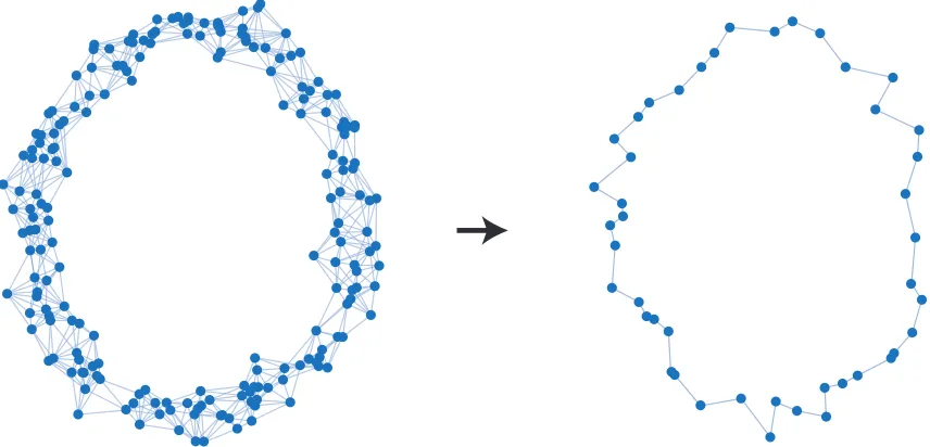
Figure 1: Network filtering based on persistent homology enables us to remove unimportant features to preserve the defining attributes represented by the network.
The metric distances between high order networks defined in Chapter 2 can be applied to com-pare networks with small number of nodes and succeed in identifying collaboration patterns of coauthorship networks. However, because they have to consider all possible node correspon-dences (Definition 1), network distances are difficult to compute when the number of nodes in the networks is large. The goal of Chapter 3 is to develop network discrimination methods that are computable in networks with large numbers of nodes. These discrimination methods are con-structed by drawing a parallel between high order networks and algebraic topology filtrations. Homological features of filtrations are then used to compare high order networks and shown to provide lower bounds for the actual network distances. Although distance lower bounds suffer from some of the same problems associated with feature comparisons, they nonetheless have im-portant properties. Among them, we know that a large lower bound entails a large distance and that we can use lower bounds to estimate distance intervals because upper bounds are easy to de-termine. The idea of using persistent homology to get lower bounds is related to the development of size theory – e.g. [33] – and the consideration of multidimensional persistent Betti numbers, see e.g. [34]. Besides, the discrete approach examined in this manuscript is not restrictive but closely related with continuous approaches considered in previous work such as [35].
filterednetwork to form a simpler and less twisting ring, like the right of Figure 1. In Chapter 4, we follow results in Chapter 3 to advocate the use of persistent homology [36, 37, 38] in such network filtering operation. It is known that more persistent homological features are more likely associated with true features, rather than artifacts of sampling or noise [38]. We leverage such charactersitic to define the frequency, spectrum, and the filter operation on networks. Our main contributions are: (i) We can define valid transforms from networks to homology frequency, and from homology frequency back to networks (Theorem 7), (ii) The difference between the original network and its filtered network is small (Theorem 8), and (iii) If we apply filter onto a pair of networks, the distance between the filtered networks well preserves the original distance between the pair (Theorem 9).
From the network distances defined in Chapter 2, we could evaluate network distance lower bound by using homological features of the corresponding network from results in Chapter 3. In the same time, network upper bounds can be easily obtained by using specific correspondence between the node spaces of the two networks. These two observations combined imply that we have both lower and upper bounds – computationally efficient – of the actual network distances, which are unknown due to computational intractability. In principal, we could cluster the space of networks using these bounds. Motivated by this, in Chapter 5 we study the clustering problem where distances between points are uncertain but known to be in an interval with lower and upper bounds. We use axiomatic approach by first defining reasonable requirements that any clustering methods in such problem should satisfy, and exploring which methods are reasonable. Clustering via distance intervals is a particular case of the problem of clustering with uncertain observations where the unpredictability is given by the distance intervals. Clustering methods that attempt to take uncertainty into consideration include the construction of models to replicate the properties of uncertainties in the data [39, 40, 41], the consideration of multiple observations of points given in a Euclidean space [42, 43, 44, 45], and the uncertainty exclusive clustering methods [46, 39, 47]. The work in Chapter 5 differs in that we investigate situations where the only available information are the upper and lower bounds of the dissimilarities. Since distance intervals can be constructed from partial information in the uncertain samples, distance intervals can be considered as a more crude observation.
It has been proved in [48] that single linkage [49, Ch. 4] is the unique hierarchical clustering method that satisfies three reasonable axioms. These results were later extended to asymmetric networks not necessarily metric, and the number of axioms required for unicity results reduced to only two [48, 21]. In the case of metric spaces the two properties that are imposed as axioms in [21] can be intuitively stated as:
(A1) Axiom of Value. Two nodes form a single cluster determined by their distance.
(A2) Axiom of Transformation. A metric space that is uniformly dominated by another metric space
should have clusters that are uniformly dominated.
1 1
11
3 3
11
5 5
11
NX a
c b
NY a
c b
NZ a
c b
-6 -4 -2 0 2 4 6
-1 0 1
a
c b
-6 -4 -2 0 2 4 6
-1 0 1
a
c b
-6 -4 -2 0 2 4 6
-1 0 1
a
c b
Figure 2: An example where different networks result in identical multi-dimensional scaling re-sults. We emphasize that the number of dimension used in multi-dimensional scaling would not distinguish networks since the triangle inequality property for relationships between nodes in the networks is violated. Such a caveat would be solved by inducing semimetrics in the space defined by the given networks, as we develop throughout Section 6.2.
for clustering based on distance intervals. To adapt condition (A1) we introduce a confidence parameter which is intended to assign different relative trusts to lower and upper bounds and require that: (A1) The nodes in a network with two nodes are clustered at the convex combination of the interval extremes dictated by the confidence parameter. Condition (A2) are then adapted correspondingly to fit in the realm of confidence parameter for distance intervals. The contribu-tions of Chapter 5 are: (i) To define thecombine-and-cluster andcluster-and-combinemethods that satisfy axioms (A1) and (A2). (ii) To prove that these methods are extremal across all methods that satisfy axioms (A1) and (A2). (iii) To demonstrate the practical applicability of the methods in the clustering of moving points via snapshots and the clustering of coauthorship networks denoting collaboration between researchers.
1.2. Applied Graph Signal Processing
In the network discrimination part of my thesis, networks are themselves the interest of analy-sis. In this second thrust, the network serves as an underlying topology describing proximities between vertices and the subject of study is a signal supported on the network [53, 54]. The pur-pose of this part of my thesis is to develop domain specific network analysis tools by leveraging the information entailed by the network in order to make apparent the presence of features that would otherwise remain occult.
As an example, consider the core task of a recommendation system which is the estimation of the rating that a user would give to a certain item. Traditionally, ratings are considered as a two dimensional matrix and the main techniques used to solve the prediction problem are matrix com-pletion [55] and collaborative filtering [56]. These methods rely on the fact that while the number of users of the system may be large there is a much smaller number of tastes. While empirical ob-servations say that this is largely true, the inherent noise in available rankings limits the precision of these tools. My approach to this problem is to use ratings and meta-information to construct a network of similarities between items. The ratings given by each user can then be viewed as a graph signal. It further follows that the ratings given by the same user should be similar if the evaluated items are highly alike with respect to the similarity measure in the constructed net-work. The information can also be used to construct an underlying network entailing proximities between user tastes, and the ratings for each item could be considered as a graph signal defined on top of this network – the exact dual by switching the roles of items and users –, and the ratings given for the same item should be similar if the users who assess them possess similar tastes. In either case, the estimation of rankings can be formulated as a low pass filtering problem. The signal that we are given is highly variable because many ratings are missing. The signal that we want is a low frequency signal where similar nodes have similar ratings.
differences, as illustrated in Figures 76 and 78, and offer other perspectives to apply graph signal processing to functional brain analytics. The theory of GSP has been growing rapidly in recent years, with development in areas including sampling theory [63, 64], stationarity [65, 66] and un-certainty [67, 68, 69, 70], filtering [71, 72, 73], directed graphs [74], and dictionary learning [75]. Applications have been spanning many areas including neuroscience [76, 77], imaging [78, 79], medical imaging [80], video [81], online learning [82], and rating prediction [83, 84, 85, 86, 87].
After introducing notations and definitions of GSP in Chapter 7, we start the Part II in Chapter 8 by first considering signals supported on graphs and addressing the challenge of defining a notion of distance between these signals that incorporates the structure of the underlying network. We want these distances to be such that two signals are deemed close if they are themselves close – in the examples in the previous paragraph we have gene expression or brain activation patterns that are similar –, or if they have similar values in adjacent or nearby nodes – the expressed genes or the active areas of the brain are not similar but they effect similar changes in the gene network or represent activation of closely connected areas of the brain. We define here the diffusion and superposition distances and argue that they inherit this functionality through their connection to diffusion processes. Besides, in Chapter 8 we illustrate that both distances are well behaved with respect to small perturbations in the underlying network and demonstrate their value in two practical scenarios; the classification of ovarian cancer types from gene mutation profiles and the classification of handwritten arabic digits.
Advances in neuroimaging techniques such as magnetic resonance imaging (MRI) have provided opportunities to measure human brain structure and function in a non-invasive manner [88]. Diffusion-weighted MRI allows to measure major fiber tracts in white matter and thereby map the structural scaffold that supports neural communication. Functional MRI (fMRI) takes an indirect estimate of the brain approximately each second, in the form of blood oxygenation level-dependent (BOLD) signals. An emerging theme in computational neuroimaging is to study the brain at the systems level with such fundamental questions as how it supports coordinated cog-nition, learning, and consciousness.
Shaped by evolution, the brain has evolved connectivity patterns that often look haphazard yet are crucial in cognitive processes. The apparent importance of these connectomes, has motivated the emergence of network neuroscience as a clearly defined field to study the relevance of network structure for cognitive function [89, 90, 91]. The fundamental components in network neuroscience are graph models [92] where nodes are associated to brain regions and edge weights are associated with the strength of the respective connections. This connectivity structure can be measured directly by counting fiber tracts in diffusion weighted MRI or can be inferred from fMRI BOLD measurements. In the latter case, networks are said to be functional and represent a measure of co-activation, e.g., the pairwise Pearson correlation between the activation time series of nodes. Functional connectivity networks do not necessarily represent physical connections although it has been observed that there is a strong basis of anatomical support for functional networks [93].
of tools from graph theory and network science [92]. These analyses have uncovered a variety of measures that reflect organizational principles of brain networks such as the presence of commu-nities where groups of regions are more strongly connected between each other than with other communities [93, 94]. Network analysis has also been related to behavioral and clinical mea-sures by statistical methods or machine learning tools to study development, behavior, and ability [95, 96, 97].
As network neuroscience expands from understanding connectomes into understanding how con-nectomes and functional brain activity support behavior, the study ofdynamicshas taken center stage. In addition, there is a rise of interest in analyzing and understanding dynamics of functional signals and with them, network structure. Such changes happen at different timescales, from years – e.g., in developmental studies [98] – down to seconds within a single fMRI run of several min-utes [99], or following tasks such as learning paradigms [97, 62, 76]. So far, common approaches include examining changes in network structure (e.g., reflecting segregation and integration) [100] or investigating time-resolved measures of the underlying functional signals [101, 102, 103]. In the case of developmental studies, the evolution of structural networks is important, but large-scale anatomical changes do not occur in the shorter time scales that are involved in behavior and ability studies. In the latter case, the notion of a dynamic network itself makes little sense and the more pertinent objects of interest are the dynamic changes in brain activity signals [62, 76]. Inasmuch as brain activity is mediated by physical connections, the underlying network structure must be taken into account when studying these signals. Tools from the emerging field of GSP are tailored for this purpose. We have applied such tools to analyze fMRI signals on top of the brain networks denoting functional connectivity (Chapter 9) as well as the brain networks quantifying structural connectivity (Chapter 10).
For brain networks denoting functional similarity between pairs of brain regions as in Chapter 9, we applied graph frequency analysis to a group of subjects try to learn a visual task. The most important observations are: (i) In terms of changes throughout the learning process, at the start of the task, BOLD signals concentrate on graph high frequency components; at the end of the task, BOLD signals concentrate on graph low frequency components; such change is significant. (ii) In terms of contribution to better learning performance, at the start of learning, BOLD signals concentrating on graph low frequency entail better learning performance; at the end of learning, BOLD signals concentrating on graph high frequency imply better learning performance; such change in association is significant as well.
Finally, GSP tools can also be used to predict unknown in modern recommendation systems. Widespread deployment of Internet technologies has generated massive enrollment of online cus-tomers in web services, propelling the emergence of recommendation systems to assist cuscus-tomers in making decisions [104, 105]. Recommendation systems use ratings that customers have given to specific products they have consumed to predict the ratings that similar users would give to similar products. In making these predictions, recommendation systems exploit product similari-ties and the closeness of user preferences, both of which can be inferred from information that is exogenous or endogenous to the system. The most popular exogenous information approach is content filtering, which starts by defining a set of features that characterize users and items and then uses those to perform predictions on the unrated items [104, 105]. The most popular en-dogenous information approach is collaborative filtering, which relies on past user behavior and carries out predictions without defining a priori set of features. Although collaborative filtering comes with certain disadvantages (in particular when rating new products or users), it typically requires less assumptions than content filtering and yields a superior performance in real datasets [105]. As a result, it has emerged as the central approach for recommendation systems.
The two main techniques to design collaborative filtering algorithms are nearest neighbors (NN) estimators and latent linear factor (LF) models. User-based NN schemes work under the assump-tion that users who are similar tend to give similar ratings for the same product and proceed in two phases. In the first phase they use a pre-specified similarity metric to compute a similarity score for each pair of users. To avoid over-fitting and simplify computations, only similarities that exceed a threshold are considered, thereby producing a sparse graph of user similarity scores [106]. In the second phase, the unknown ratings for a particular user are obtained by combining the ratings that similar users have given to the unrated items as dictated by the similarity graph. Likewise, item-based NN approaches work under the assumption that similar products receive similar ratings and create a product similarity graph to assign ratings to unrated products.
LF approaches bypass notions of user or product similarity by posing the existence of a num-ber of latent factors that generate the user-item rating function. The main difference relative to content-filtering approaches is that here the factors are not defined a priori, but inferred from the available ratings. Although nonlinear latent factor models exist, the linear models based on ma-trix factorization (aka mama-trix completion methods [107]) combine tractability with good practical performance [105]. In particular, by arranging the available ratings in a matrix form with one of the dimensions corresponding to users and the other one to items, LF schemes typically carry out a low-rank singular value decomposition (SVD) that jointly maps users and items to a latent factor linear space of reduced dimensionality [105]. The rating user-item function is then modeled simply as inner products in the reduced subspace defined by the SVD.
a graph filter. Moreover, matrix factorization methods can be reinterpreted as interpolation al-gorithms that, given a subset of signal observations (ratings), recover the full signal under the assumption that the ratings are bandlimited in a particular spectral domain. This interpretation not only provides a better understanding on the differences and similarities between the two approaches, but it also opens the door to the design of more advanced algorithms leading to a better recommendation accuracy. In a nutshell, the contributions of Chapter 11 are: (i) To demon-strate how the standard collaborative filtering approaches based on NN and LF can be interpreted as particular types of GSP algorithms that model the rating signal as bandlimited. (ii) To ex-ploit this interpretation to design more general algorithms for NN and LF. (iii) To show that the proposed methods indeed produce significant improvement regarding rating prediction accuracy in the publicly available MovieLens 100k dataset [108]. (iv) To identify and discuss interesting observations found when using this GSP approach, which can be leveraged in the design of fu-ture recommendation system algorithms. Relative to existing contributions dealing with graph SP schemes for two-dimensional rating prediction [83, 109, 87], the work in this paper is more comprehensive, provides novel insights and puts forth new algorithms. More specifically, in the context of LF models, [83] formulates a low-rank matrix completion problem augmented with a regularizer term that promotes smoothness of the predicted ratings on the similarity graph. In comparison, our work proposes a bandlimited sampling implementation, where we separate the estimation of the frequency components (singular vectors) from the estimation of frequency coef-ficients (singular values) of the rating matrix; this separation allows for more general interpolators and reduces the computational complexity, see Section 11.4.1. In the context of NN prediction, [109] uses a pre-determined low-pass graph filter to predict ratings. In comparison, this work pos-tulates more flexible graph filters, finds the optimal (band-stop) filter coefficients in the training phase, and introduces graph filters that operate in both the user and the item domain. Finally, [87], which was published after the submission of this manuscript, uses similarity graphs and graph SP to extract local spatial features from the observed ratings, and then feeds the extracted features into a recurrent neural network to diffuse entries to reconstruct the rating matrix. Our work uses graph SP to find the optimal higher order band-stop filter via training, and to separate the estimation of singular vectors from the estimation of singular values of the rating matrix.
1.3. Published Results
Part I
Chapter 2
Network Comparison via
Correspondence
The main problem addressed in this chapter is the construction of metric distances between high order networks. Formal definitions of high order networks are presented (Section 2.2) as a gen-eralization of pairwise networks (Section 2.1). Dissimilarity networks (Section 2.3) and proximity networks (Section 2.4) are specific high order networks where relationship functions are intended to encode dissimilarities or proximities between members of tuples. Dissimilarity networks are characterized by the order increasing property which states that tuples become more dissimilar when members are added to a group. Proximity networks abide to the order decreasing property which states that tuples becomes less similar when adding nodes to the group. Two families of proper metric distances are then defined in the respective space of dissimilarity (Section 2.3.1) and proximity (Section 2.4.1) networks modulo permutation isomorphisms. These distances are built as generalizations of the pairwise distances in [21], which are themselves generalizations of the Gromov-Hausdorff distance between metric spaces [129, 130]. We also establish a duality between dissimilarity and proximity networks and the different metrics (Section 2.4.2). We use the proximity network distances defined in the chapter to compare the coauthorship networks of two popular signal processing researchers and show that they succeed in discriminating their collaboration patterns (Section 2.5).
2.1. Pairwise Networks
Conventionally, a network is defined as a pair NX = (X,r1X), where X is a finite set of nodes
and r1X : X2 = X×X → R+ is a function that may encode similarity or dissimilarity between elements. For pointsx,x0 ∈ X, values of this function are denoted asr1X(x,x0). We assume that
r1X(x,x0) =0 if and only ifx =x0 and we further restrict attention to symmetric networks where
When defining a distance between networks we need to take into consideration that permutations of nodes amount to relabelling nodes and should be considered as same entities. We therefore say that two networks NX = (X,r1X) and NY = (Y,rY1) are isomorphic whenever there exists a
bijectionπ:X→Ysuch that for all pointsx,x0 ∈X,
r1X(x,x0) =rY1(π(x),π(x0)). (2.1)
Such a map is called an isometry. Since the map π is bijective, (2.1) can only be satisfied when
X is a permutation of Y. When networks are isomorphic we write NX ∼= NY. The space of
networks where isomorphic networks NX ∼= NY are represented by the same element is termed
the set of networks modulo isomorphism and denoted by N mod ∼=. The space N mod ∼=
can be endowed with a valid metric [21]. The definition of this distance requires introducing the prerequisite notion of correspondence [131, Def. 7.3.17].
Definition 1 A correspondence between two sets X and Y is a subset C⊆X×Y such that∀x∈ X, there
exists y ∈ Y such that(x,y) ∈ C and∀y ∈ Y there exists x ∈ X such that (x,y) ∈ C. The set of all
correspondences between X and Y is denoted asC(X,Y).
A correspondence in the sense of Definition 1 is a map between node sets XandYso that every element of each set has at least one correspondent in the other set. Correspondences include permutations as particular cases but also allow for the mapping of a single point inXto multiple correspondents inY or, vice versa. Most importantly, this allows definition of correspondences between networks with different numbers of elements. We can now define the distance between two networks by selecting the correspondence that makes them most similar as we formally define next.
Definition 2 Given two networks NX = (X,r1X)and NY = (Y,r1Y)and a correspondence C between the node spaces X and Y define the network difference with respect to C as
Γ1
X,Y(C):= max
(x1,y1),(x2,y2)∈C r
1
X(x1,x2)−r1Y(y1,y2)
. (2.2)
The network distance between networks NXand NYis then defined as
d1N(NX,NY):= min
C∈C(X,Y)
n Γ1
X,Y(C)
o
. (2.3)
For a given correspondenceC∈ C(X,Y)the network differenceΓ1X,Y(C)selects the maximum dis-tance difference|r1X(x1,x2)−r1Y(y1,y2)|among all pairs of correspondents – we comparer1X(x1,x2)
with r1Y(y1,y2) when the points x1 and y1, as well as the points x2 and y2, are correspondents.
if the networks are isomorphic [21]. For future reference, the notions of metric and pseudometric are formally stated next.
Definition 3 Given a space S and an isomorphism ∼=, a function d : S × S → R is a metric in S
mod ∼=if for any a,b,c∈ S the function d satisfies:
(i)Nonnegativity. d(a,b)≥0.
(ii)Symmetry. d(a,b) =d(b,a).
(iii)Identity. d(a,b) =0if and only if a∼=b.
(iv)Triangle inequality. d(a,b)≤d(a,c) +d(c,b).
The function is a pseudometric inS mod ∼=if for any a,b,c ∈ S the function d satisfies (i), (ii), (iv),
and
(iii’)Relaxed identity. d(a,b) =0if a∼=b.
A metricdin S mod ∼=gives a proper notion of distance. Since zero distances imply elements being isomorphic, the distance between elements reflects how far they are from being isomorphic. Pseudometrics are relaxed since elements not isomorphic may still have zero distance measured by the pseudometrics. The distance in Definition 2 is a metric in spaceN mod ∼=. Observe that since correspondences may be between networks with different number of elements, Definition 2 defines a distance d1
N(NX,NY) when the node cardinalities |X| and |Y| are different. In the
particular case when the functionsr1Xsatisfy the triangle inequality, the set of networksN reduces to the set of metric spaces M. In this case the metric in Definition 2 reduces to the Gromov-Hausdorff (GH) distance between metric spaces. The distances d1N(NX,NY) in (2.3) are valid
metrics even if the triangle inequalities are violated byr1Xorr1Y[21].
In this chapter we consider high order networks where the specification of functionsrk
X :Xk+1→
R+are meant to encode similarities or dissimilarities between node(k+1)-tuples. The goal of this chapter is to devise generalizations of Definition 2 to high order networks and to prove that they define valid metrics in the space of high order networks modulo isomorphism; see Definitions 11, 12, 14, and 15.
2.2. High Order Networks
A network of order K over the node space X is defined as a collection of K+1 relationship functions{rkX:Xk+1→R+}kK=0from the spaceXk+1of(k+1)-tuples to the nonnegative reals,
NXK=
X,r0X,r1X, . . . ,rKX
. (2.4)
When some nodes are repeated in the point collectionx0:k:= (x0,x1, . . . ,xk)∈Xk+1, the
relation-ship functionrkX(x0:k)entails the same information as the relationship function between the largest
non-repeating subtuple of x0:k. In future definitions, it would be important to take the number
of distinct elements of a tuple into consideration. We formalize this property by introducing the notion of the rank of tuples as we formally specify next.
Definition 4 The rank s(x0:k)of a given tuple x0:kis the number of unique elements in the tuple.
It follows from Definition 4 that the ranks(x,x) =1 and that the ranks(x0,x,x0) = 2. Moreover, the relationship function between a tuplex0:kis identical to the relationship functions of subtuples
ofx0:kthat have same rank ass(x0:k)since they imply same information. This remark along with
a symmetry property makes up the formal definition of high order networks that we introduce next.
Definition 5 NK
X = X,r0X,r1X, . . . ,rKX
is a K-order network if the following two properties holds:
Symmetry. For any0≤k≤K and any point collections x0:k, we have that
rkX(x[0:k]) =rkX(x0:k), (2.5)
where x[0:k]= ([x0],[x1], . . . ,[xk])is a reordering of x0:k := (x0,x1, . . . ,xk).
Identity. For any0≤k≤K and tuple x0:k, any of its subtuple xl0:lk˜ with s(x0:k) =s(xl0:lk˜)satisfies
rkX(x0:k) =r ˜ k
X(xl0:lk˜). (2.6)
The set of all high order networks of order K is denoted asNK.
For point collectionsx0:k, values of theirk-order relationship functions are denoted asrkX(x0:k)and
are intended to represent a measure of similarity or dissimilarity for members of the group. In particular, the zeroth order function r0X encodes relative weights of different nodes and the first order functionr1
X represents the pairwise information discussed in Section 2.1. Observe however
that pairwise networks are not particular cases of networks of order 1 because a network of order
Knot only requires the definition of relationships between(K+1)-tuples but also of relationships between (k+1)-tuples for all integers 0 ≤ k ≤ K. A network of order 0 is one in which only node weights are given, a network of order 1 is one in which weights and pairwise relationships are defined, a network of order 2 adds relationships between triplets and so on. Examples for the identity property includes r2X(x,x) = r1X(x) and r3X(x0,x,x0) = r2X(x,x0). We assume that relationship values are normalized so that 0 ≤ rk
X(x0:k) ≤ 1 for all kand x0:k. As in the case of
Definition 6 We say that two networks NXKand NYKare k-isomorphic if there exists a bijectionπ:X→Y
such that for all x0:k∈Xk+1we have
rkY(π(x0:k)) =rkX(x0:k), (2.7)
where we use the shorthand notation rYk(π(x0:k)):=rkY(π(x0),π(x1), . . . ,π(xk)). The mapπis called a
k-isometry.
When networksNK
XandNYKarek-isomorphic we writeNXK∼=k NYK. The space ofK-order networks
modulo k-isomorphism is denoted byNK mod ∼=
k. For each nonnegative integer 0 ≤ k ≤ K,
the spaceNK mod ∼=
k of networks of order K modulok-isomorphism can be endowed with a
pseudometric. The definition of this family of pseudometrics is a generalization of Definition 2 as we formally state next.
Definition 7 Given networks NXKand NYK, a correspondence C between the node spaces X and Y, and an
integer0≤k≤K define the k-order network difference with respect to C as
Γk
X,Y(C):= max
(x0:k,y0:k)∈C
r
k
X(x0:k)−rkY(y0:k)
, (2.8)
where the notation(x0:k,y0:k)stands for(x0,y0),(x1,y1), . . . ,(xk,yk). The k-order network distance
be-tween networks NXKand NYKis then defined as
dkN(NXK,NYK):= min
C∈C(X,Y)
n Γk
X,Y(C)
o
. (2.9)
We further define the K-order distance vector as the K+1dimensional vectordKN(NXK,NYK) =
d0N(NXK,NYK), . . . ,
dK
N(NXK,NYK)
T
that groups the k-order distances in(2.9).
Both, Definition 2 and Definition 7 consider correspondencesCthat map the node spaceXonto the node space Y, compare dissimilarities, and set the network distance to the comparison that yields the smallest value in terms of maximum differences. The distinction between them is that in (2.2) we compare the values inr1X(x1,x2)andrY1(y1,y2), whereas in (2.8) we compare the
values in each of thek-order relationships rk
X(x0:k)andrkY(y0:k)to compute thek-order distances dkN(NXK,NYK) that we group in the vector dKN(NXK,NYK). Except for this distinction, Definition 2 and Definition 7 are analogous sinceΓkX,Y(C)selects the maximumk-order relationship difference |rkX(x0:k)−rkY(y0:k)|among all tuples of correspondents – we comparerkX(x0:k)withrkY(y0:k)when
all the pointsxl ∈ x0:kand yl ∈ y0:k are correspondents. The distancedkN(NXK,NYK)is defined by
selecting the correspondence that minimizes these maximal differences.
1 1
1
1
C
C
C N1
X
x1
1
x2
1 x3 1
N1
Y
y1 1
y2
1
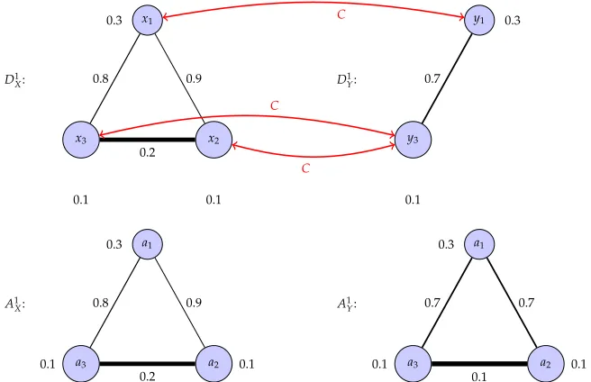
Figure 3: An example of two networks being not 1-isomorphic but having zero 1-order network distance between them. For the given correspondence C, r2X(x1,x2) = r2Y(y1,y2), r2X(x1,x3) = r2Y(y1,y2). r2X(x2,x3) = rY2(y2,y2) = r1Y(y2) where the second equality follows from the
iden-tity property. Moreover, r2X(x1,x1) = r2Y(y1,y1), r2X(x2,x2) = r2Y(y2,y2), r2X(x3,x3) = r2Y(y2,y2).
Γ1
X,Y(C) = 0 witnesses the zero 1-order network distance between NX1 and NY1. However these
networks cannot be 1-isomorphic since they possess different number of nodes.
dkN(NXK,NYK)anddNK(NXK,NYK)are defined even if the numbers of nodes inXandYare different. We show in the following proposition that the function dkN : NK× NK → R
+ is, indeed, a pseudometric in the space ofK-order networks modulok-isomorphism for any integer 0≤k≤K.
Proposition 1 Given any nonnegative integer K, for any integers0 ≤ k≤ K, the function dkN :NK×
NK→R
+defined in (2.9) is a pseudometric in the spaceNK mod ∼=k.
Proof: To prove thatdkN for any integer 0≤k≤Kis a pseudometric in the space ofK-order net-works modulok-isomorphism we prove the (i) nonnegativity, (ii) symmetry, (iii’) relaxed identity, and (iv) triangle inequality properties in Definition 3.
Proof of nonnegativity property: For any integers 0≤k≤K, since|rkX(x0:k)−rYk(y0:k)|is
non-negativeΓkX,Y(C)defined in (2.8) also is. The network distance must then satisfydkN(NXK,NYK)≥0
because it is a minimum of nonnegative numbers.
Proof of symmetry property: A correspondence C ⊆ X×Y with elements ci = (xi,yi)
re-sults in the same associations as the correspondence ˜C ⊆ Y×X with element ˜ci = (yi,xi).
Thus, for any correspondence C and integers 0 ≤ k ≤ K, we have a correspondence ˜C such thatΓkX,Y(C) =ΓkY,X(C˜). It follows that the minima in (2.9) must coincide from where it follows
thatdkN(NXK,NYK) =dkN(NYK,NXK).
Proof of relaxed identity property: We need to show that for any integers 0 ≤ k ≤ K if NXK
and NK
Y are k-isomorphic we must have dkN(NXK,NYK) = 0. To see that this is true recall that for k-isomorphic networks there exists a bijection π : X → Y that preserves distance functions at orderk[cf. (2.7)]. Consider then the particular correspondenceCπ ={(x,π(x)),x ∈ X}. For all x0∈Xthere is an elementc= (x0,y)∈Cπand for ally0∈Ythere is an elementc0= (x,y0)∈Cπ
that it must be
rYk(y0:k) =rYk(π(x0:k)) =rkX(x0:k), (2.10)
for any(x0:k,y0:k)∈Cπ. This impliesΓkX,Y(C) =
rkX(x0:k)−rkY(y0:k)
=0 for any(x0:k,y0:k)∈Cπ.
SinceCπ is a particular correspondence, taking a minimum over all correspondences as in (2.9)
yields
dkN(NXK,NYK)≤Γk
X,Y(C) =0. (2.11)
Sincedk
N(NXK,NYK)≥0, as already shown, it must be thatdkN(NXK,NYK) =0 when NXKand NYK are
k-isomorphic.
Proof of triangle inequality: To show that the triangle inequality holds, let the correspondenceC1
betweenXandZand the correspondenceC2betweenZandYbe the minimizing correspondences
in (2.9). We can then write
dkN(NXK,NZK) =ΓkX,Z(C1), dkN(NZK,NYK) =ΓkZ,Y(C2). (2.12)
Define a correspondenceCbetweenXandYas the one induced by pairs(x,z)and(z,y)sharing a common nodez∈Z,
C:={(x,y)| ∃z∈Zwith(x,z)∈C1,(z,y)∈C2}. (2.13)
To show that C is a well defined correspondence we need to show that for every x ∈ X there existsy0∈Ysuch that(x,y0)∈Cand by symmetry for everyy∈Ythere existsx0∈Ysuch that (x0,y) ∈ C. To see this, first pick an arbitrary x ∈ X. Because C1 is a correspondence between X and Z there must exist z0 ∈ Z such that (x,z0) ∈ C1. There must exist y0 ∈ Y such that (z0,y0) ∈ C2 since C2 is also a correspondence betweenY and Z. Therefore, there exists a pair (x,y0) ∈ T with y0 ∈ Y for any x ∈ X. The second part follows by symmetry and C is a well
defined correspondence. The correspondenceC may not be the minimizing correspondence for the distancedkN(NXK,NYK). However since it is a valid correspondence with the definition in (2.9) we can write
dkN(NXK,NYK)≤ΓkX,Y(C). (2.14)
By the definition ofCin (2.13), the requirement(x0:k,y0:k)∈Cis equivalent as(x0:k,z0:k)∈C1and (z0:k,y0:k)∈C2for any 0≤k≤K. Further adding and subtractingrkZ(z0:k)in the absolute value
ofΓkX,Y(C) =
rkX(x0:k)−rkY(y0:k)
and using the triangle inequality of the absolute value yields
Γk
X,Y(C)≤ max
(x0:k,z0:k)∈C1 (z0:k,y0:k)∈C2
n
rkX(x0:k)−rkZ(z0:k) +
rkZ(z0:k)−rkY(y0:k) o
We can further bound (2.15) by taking maximum over each summand,
Γk
X,Y(C) ≤ max
(x0:k,z0:k)∈C1
rkX(x0:k)−rkZ(z0:k) +
max (z0:k,y0:k)∈C2
rkZ(z0:k)−rYk(y0:k)
=ΓkX,Z(C1) +ΓkZ,Y(C2). (2.16)
Substituting (2.14) and (2.12) into (2.16) yields triangle inequality.
Having proofs all statements, the global proof completes.
dkN being a pseudometric implies that two high order networks notk-isomorphic may still have zerok-order network distance between them. A specific example can be found in Figure 3 where two 1-order networks not 1-isomorphic have zero dissimilarity measured by the 1-order network distance. For each integer 0≤k≤K, the pseudometricdkN(NXK,NYK)defined in Definition 7 in the spaceNK mod ∼=
k measures dissimilarity betweenk-order functionsrkX andrYk. We can also ask
the question of how different two networks are by considering alltheir order functions. To that end we consider K-order networks to be equivalent ifrkX is a permutation of rkX for all integers 0≤k≤Kas we formally state next.
Definition 8 We say that two networks of order K, NXKand NYK, are isomorphic if there exists a bijection
π:X→Y such that(2.7)holds for all0≤k≤K and x0:k∈Xk+1. The mapπis called an isometry.
When networks NXK and NYK are isomorphic we write NXK ∼= NYK. The difference between k -isomorphism and -isomorphism is that the bijection in the latter case preserves relationship func-tions over all orders whereas onlyk-order relationship functions are preserved in the former case. That NXK ∼= NYK implies that NXK ∼=k NYK for all integers 0 ≤ k ≤ K, but the opposite is not
necessarily true.
The space of K-order networks modulo isomorphism is denoted as NK mod ∼=. A family of pseudometrics measuring the difference between networks over all order functions as a whole can be endowed in the spaceNK mod ∼=. The definition of this family of distances can be considered as an extension of Definition 2 and an aggregation of Definition 7 as we formally state next.
Definition 9 Given networks NXK and NYK, a correspondence C between the node spaces X and Y, and
some p-normk · kp, define the network difference with respect to C as
Γ
K
X,Y(C)
p:=
Γ0
X,Y(C),Γ1X,Y(C), . . . ,ΓKX,Y(C)
T
p, (2.17)
where for each integer0 ≤ k≤ K,ΓkX,Y(C)is the k-order network difference with respect to C defined in
(2.8). The p-norm network distance between NXKand NYKis then defined as
dN,p(NXK,NYK):= min
C∈C(X,Y)
Γ
K
X,Y(C)
p
The difference between Definition 2, Definition 7 and Definition 9 is that in the case of the network distancedN,p(NXK,NYK), we compare not only relationship functionsrkX(x0:k)andrYk(y0:k)but also
all the relationship functions of order not larger thanK. The norm over the vectorΓKX,Y(C)formed by k-order network differences with respect to C for all integers 0 ≤ k ≤ K is assigned as the difference between NXK and NYK measured by the correspondence C. The distancedN,p(NXK,NYK)
is then defined as the minimum of these differences achieved by some correspondence. As in the cases of Definition 2 and Definition 7,dN,p(NXK,NYK) is defined even if the numbers of nodes in X and Y are different. The function dN,p : NK× NK → R+ is a pseudometric in the space of
K-order networks modulo isomorphism as we show in the following proposition.
Proposition 2 Given some p-normk · kp, for any nonnegative integer K the function dN,p:NK× NK→
R+defined in (2.18) is a pseudometric in the spaceNK mod ∼=.
Proof: To prove that dN,p is a distance in the space ofK-order networks modulo isomorphism
we prove the (i) nonnegativity, (ii) symmetry, (iii’) relaxed identity, and (iv) triangle inequality properties in Definition 3.
Proof of nonnegativity property: SincekΓK
X,Y(C)kp ≥0, the network distance must then satisfy dN,p(NXK,NYK)≥0 as it is a minimum of nonnegative numbers.
Proof of symmetry property: A correspondenceC ⊆ X×Y with elementsci = (xi,yi)results
in the same associations as the correspondence ˜C ⊆ Y×X with element ˜ci = (yi,xi). Thus,
for any correspondence C we have a correspondence ˜C such that ΓKX,Y(C) = ΓKY,X(C˜). This im-plieskΓK
X,Y(C)kp =kΓKY,X(C˜)kp. It follows that the minima in (2.18) must coincide and therefore
dN,p(NXK,NYK) =dN,p(NYK,NXK).
Proof of relaxed identity property: We need to show that ifNK
X andNYKare isomorphic we must
havedN,p(NXK,NYK) = 0. To see that this is true recall that for isomorphic networks there exists
a bijectionπ : X →Y that preserves distance functions at every order [cf. (2.7)]. Consider then the particular correspondence Cπ = {(x,π(x)),x ∈ X}. We have demonstrated in the proof of
Proposition 1 thatCπ is a valid correspondence betweenXandY. The definition of isomorphism
indicates that it must be (2.10) holds true for all 0 ≤ k ≤ K and (x0:k,y0:k) ∈ Cπ. SinceCπ is a
particular correspondence, from (2.18) it follows that
dN,p(NXK,NYK)≤
Γ
K
X,Y(C)
p. (2.19)
Because rkX(x0:k)−rkY(y0:k) = 0 for any 0 ≤ k ≤ K and any (x0:k,y0:k) ∈ Cπ by (2.10), we have ΓK
X,Y(C) = 0. k · kp being a proper norm implies kΓKX,Y(C)kp = 0. Substituting this back into
(2.19) shows dN,p(NXK,NYK) ≤ 0. Since dN,p(NXK,NYK) ≥ 0, as already shown, it must be that dN,p(NXK,NYK) =0 whenNXKand NYKare isomorphic.
betweenXandZand the correspondenceC2betweenZandYbe the minimizing correspondences
in (2.18). We can then write
dN,p(NXK,NZK) =
ΓKX,Z(C1)
p, dN,p(NZK,NYK) =
ΓKZ,Y(C2)p. (2.20)
Define a correspondenceCbetweenXandYin the same way as (2.13). We have demonstrated in the proof of Proposition 1 thatCis a well defined correspondence. Therefore with the definition in (2.18) we can write
dN,p(NXK,NYK)≤
ΓKX,Y(C)
p. (2.21)
Moreover, in the proof of Proposition 1 we also showed for any 0≤k≤K,
Γk
X,Y(C)≤ΓkX,Z(C1) +ΓkZ,Y(C2). (2.22)
This implies the vectorΓKX,Z(C1) +ΓKZ,Y(C2)is elementwise no smaller than the vectorΓKX,Y(C). The
definition of p-normkxkp = ∑Kk=0|xi|p
1/p
guarantees that the value of kxkp is monotonically
nondecreasing on each elementxiinx= (x0,x1, . . . ,xn)T. Therefore,
Γ
k
X,Y(C)
p≤ Γ k
X,Z(C1) +ΓkZ,Y(C2)
p. (2.23)
We can further bound (2.23) by using the triangle inequality of thep-norm,
Γ
k
X,Y(C)
p≤ Γ k
X,Z(C1)
p+ Γ k
Z,Y(C2)
p. (2.24)
Substituting (2.21) and (2.20) back into (2.24) yields the triangle inequality.
Having demonstrated all statements, the global proof completes.
Observe that in (2.18) we are only allowed to pick one correspondence minimizing kΓK
X,Y(C)kp
whereas in (2.9) for eachkwe are able to pick one correspondence minimizing the order specific
Γk
X,Y(C). This establishes a relationship betweendN,pandkdKNkpthat we show next.
Proposition 3 Given some p-norm k · kp, for any nonnegative integer K the function dN,p defined in
(2.18)is no smaller thankdKNkpwhere dKN is the vector of distances defined in Definition 7. I.e., for any
pair of K-order networks NK
X,NYK, we have that
dN,p(NXK,NYK)≥
d
K
N(NXK,NYK)
p. (2.25)
Proof: Given K-order networksNK
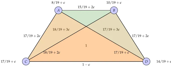
![Figure 5: Collaborations between authors in a research community.Theof publications – and the multiplication of k-order relationshipfunction in this 2-order network [cf.Definition 13] incorporates the proximity function – thenumber of publications between members of a given (k + 1)-tuples normalized by the total number −ϵ with the rank of the tuple.](https://thumb-us.123doks.com/thumbv2/123dok_us/9232215.1458775/43.612.162.490.73.205/collaborations-publications-multiplication-relationshipfunction-denition-incorporates-publications-normalized.webp)