www.atmos-meas-tech.net/8/3527/2015/ doi:10.5194/amt-8-3527-2015
© Author(s) 2015. CC Attribution 3.0 License.
Combined vertical-velocity observations with Doppler lidar, cloud
radar and wind profiler
J. Bühl1, R. Leinweber2, U. Görsdorf2, M. Radenz1, A. Ansmann1, and V. Lehmann2 1Institute for Tropospheric Research (TROPOS), Permoserstr. 15, 04318 Leipzig, Germany 2Deutscher Wetterdienst, Meteorologisches Observatorium Lindenberg (MOL),
Am Observatorium 12, 15848 Tauche, Germany
Correspondence to: J. Bühl ([email protected])
Received: 9 December 2014 – Published in Atmos. Meas. Tech. Discuss.: 12 January 2015 Revised: 8 July 2015 – Accepted: 25 July 2015 – Published: 31 August 2015
Abstract. Case studies of combined vertical-velocity mea-surements of Doppler lidar, cloud radar and wind profiler are presented. The measurements were taken at the Meteorologi-cal Observatory, Lindenberg, Germany. Synergistic products are presented that are derived from the vertical-velocity mea-surements of the three instruments: a comprehensive classi-fication mask of vertically moving atmospheric targets and the terminal fall velocity of water droplets and ice crystals corrected for vertical air motion. It is shown that this combi-nation of instruments can up-value the measurement values of each single instrument and may allow the simultaneous sensing of atmospheric targets and the motion of clear air.
1 Introduction
Mixed-phase layered clouds are a critical component of the global weather and climate system. The occurrence of these clouds is difficult to predict, because the interaction between aerosols, cloud droplets and atmospheric dynamics is not un-derstood. Errors in the prediction of layered clouds strongly affect the accuracy of global climate projections, because of their extended global appearance (D. Zhang et al., 2010; Y. Zhang et al., 2010).
Vertical motions of different scales are important for the development and the life-cycle of layered clouds. Large-scale atmospheric motions can influence the observations of an ex-isting cloud decisively, e.g. by altering the vertical veloc-ity of falling droplets or ice crystals. Furthermore, it was shown by Korolev and Field (2008) and recently by Sim-mel et al. (2014) that turbulent motion within the cloud layer
can maintain its mixed-phase state, even if ice particles have formed that draw water vapor from the liquid droplets due to the Bergeron-Findeisen process. This large variety of scales and processes cannot be covered by a single instrument. Dif-ferent efforts have been made to combine remote-sensing instruments in order to get a detailed picture of the pro-cesses involved in such mixed-phase layered clouds on small (Wandinger et al., 2012; Bühl et al., 2012, 2013) and large scales.
the mode of operation used in the context of this paper. Even larger heights (up to 16 km) are available using a longer pulse length. The large height coverage is very important in our case, because in the mid-latitudes mixed-phase clouds most commonly occur in the height interval between 2 and 8 km (D. Zhang et al., 2010).
All three velocity-measuring instruments are most sensi-tive to particles or structures which are similar in size to the operating wavelength λof the instrument (see Table 1). The Doppler lidar (λ=1.5 µm) is most sensitive to aerosol particles (100 nm to 10 µm in diameter). The cloud radar (λ=8.5 mm) is capable of sensing cloud droplets (10 to 100 µm). Additionally it shows large signals for hydromete-ors like drizzle droplets, rain droplets or ice crystals (100 µm to 10 mm). The wind profiler detects echoes from refrac-tive index fluctuations originating from turbulent eddies in the atmosphere with sizes of half its wavelength of λ=
0.62 m and Rayleigh scattering from particles. In this work, the combined operation of this unique set of instruments is demonstrated in order to study the vertical motions in and around layered clouds. The combination of wind profiler and cloud radar has been done before (Tridon et al., 2013). Pro-tat and Williams (2011) also showed the principle of com-bined vertical-velocity observations, but with a combination of 50 MHz wind-profiler and 3 GHz radar. It is the focus of this paper to show that an additional Doppler lidar can de-liver complementary information about the vertical veloc-ity of small cloud droplets and their fast-changing turbu-lent motion. For that purpose, first tentative efforts of the MOL/TROPOS measurement campaign COLRAWI (Com-bined Observations with Lidar, Radar and Wind Profiler) are presented here. It is shown that turbulent air motion, large-scale waves and the vertical movement of falling ice and water particles can be measured at once. In this way a co-herent picture of different kinds of vertical motions in the atmosphere can be drawn and the unbiased fall velocity of particles can be measured.
This paper deals with first promising examples how to combine Doppler lidar, cloud radar and wind profiler. In Sect. 2 an overview is given about the three instruments and their simultaneous operation. In Sect. 3, case studies are pre-sented and links between the data from the different instru-ments are established. A summary is given in Sect. 4.
2 Overview about measurement instruments and strategy
Wind-profiler radars have been designed to measure the wind speed in both the cloudy and clear atmosphere. While the radar technique itself is nearly 70 years old, the wind profiler technique was not developed before the 1970s (Woodman and Guillen, 1974; Strauch et al., 1984; Weber and Wuertz, 1990). A wind profiler exploits Bragg scattering at atmo-spheric density fluctuations to produce a backscatter signal
Figure 1. Aerial view of the wind profiler site at MOL. The
photo-graph was taken in September 2011. In the meantime a Streamline Doppler lidar and a MIRA-35 cloud radar were deployed next to the wind profiler. During the measurements presented here, all instru-ments were pointing vertical at all times. Operational parameters of the systems measuring vertical velocity can be found in Table 1. (Bühl, 2015)
even under clear-air conditions. Rayleigh and Bragg scatter-ing is proportional toλ−4andλ−13, respectively.
Hence, Bragg scattering dominates more and more for longer wavelengths, but Rayleigh scattering from particles can still add to the signal. This Rayleigh-Bragg ambiguity limits the measurement of air motions in the presence of par-ticles (Gage et al., 1999; Knight and Miller, 1998). Since particles are always falling with a certain velocity relative to the surrounding air, a bias towards negative velocities oc-curs, e.g., within cloud layers or rain. In Sect. 3.5 an outlook is given on a possible method to reduce this bias for the com-bination of cloud radar and wind profiler at MOL.
The distribution of powerful wind profilers is limited, but they can actually deliver the desperately needed information about the velocity of clear air. The DWD operates a UHF wind profiler at MOL (see Fig. 1). It works at 482 MHz and can deliver wind information from 0.5 km to a maximum of 16 km height with a range resolution of 150 m and a mea-surement interval of about 10 s (Böhme et al., 2004). The dis-tance between two neighboring range gates is 100 m, due to range oversampling. Usually, the wind profiler is operated to derive the height-resolved horizontal wind with a four-beam Doppler beam-swinging technique. For the duration of the measurements presented here, Doppler lidar, cloud radar and wind profiler were always used in a vertical-stare mode.
Table 1. Technical properties of the three main instruments involved in the combined measurements.
Designation Doppler lidar UHF Wind profiler Cloud radar
System type HALO Streamline LAP 16000 MIRA-35
Wavelength 1.5 µm 0.62 m 8.5 mm
Pulse width 160 ns 1000 ns 200 ns
Range gate length 48 m 94 m 30 m
Integration time 2 s 10 s 10 s
Beam width 0.05 mrad 50 mrad 10 mrad
Pulse repetition rate 15 kHz 12.2 kHz 5 kHz Average emitted power 200 mW 200 W 30 W
particle sizes. For droplets and ice crystals the Doppler lidar is operating in the geometrical optics regime and the signal response is proportional to the square of the particle diame-terD. That makes the Doppler lidar especially sensitive for aerosol particles and cloud droplets. The cloud radar, on the other hand, operates in the Rayleigh regime due to its longer wavelength and is sensitive toD6. The cloud radar signal is therefore easily dominated by larger particles in the obser-vation volume, i.e., ice crystals or rain droplets. Within the context of this work, vertical velocity from cloud radar is al-ways the reflectivity-weighted vertical velocity, i.e. the first moment of the cloud radar spectrum at a given range gate. Therefore, this value is mainly representing the vertical mo-tion of the largest particles within the observamo-tion volume.
Hence, a combination of Doppler lidar, cloud radar and wind profiler enables the observation of a large variety of motions within the atmosphere from the turbulence within cloud layers, over the fall speed of large ice crystals towards the motion of air itself.
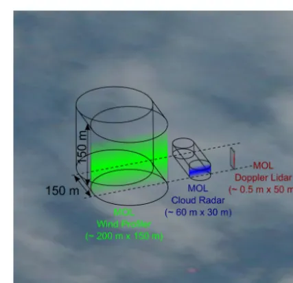
Table 1 shows the operational parameters of the main in-struments for combined measurements of vertical velocity at MOL. All systems were co-located within a 30 m radius (see Fig. 1) and had therefore overlapping observation vol-umes. A schematic representation of the observation volumes is given in Fig. 2 illustrating the large technical differences between the three systems. In the context of this work, the Doppler lidar is operated with a measurement interval of 2 s, cloud radar and wind profiler both with 10 s. The resolution of vertical velocity of all three instruments presented here is below 0.1 m s−1. Signal processing, noise filtering and error estimations for Doppler lidar, cloud radar and wind profiler can be found in Pearson et al. (2009); Görsdorf et al. (2015) and Lehmann (2012); Angevine (1997), respectively. In the following, different case studies are presented to demonstrate the manifold of possibilities enabled by this new combination of instruments.
3 Case studies
A combined vertical-velocity measurement with Doppler li-dar, cloud radar and wind profiler from 30 July 2013 is shown
Figure 2. Comparison of observation volumes of Doppler lidar
(red), cloud radar (blue) and wind profiler (green). Beam diame-ter times folded pulse length is given in brackets below the sys-tem names. The length interval of 150 m, indicated by two dashed lines, is the displacement of the cloud during an integration time of 10 s, when moving with an advection speed of 15 m s−1. In the background, a representation to scale of the altocumulus at 4000 m height is shown. In this figure, only the sizes of the observation volumes are shown. In reality, the observation volumes of cloud radar and Doppler lidar would overlap from about 1000 m height upwards. One pulse of the wind profiler fills a factor of 104. . .105 more space than the Doppler lidar.
in Fig. 3. In the following Section different parts of this scene will be analyzed with respect to different aspects of vertical motions in the atmosphere.
V
er
tical
V
el
ocity [
m
s
⁻
¹]
He
ig
ht
[m
]
He
ig
ht
[m
]
He
ig
ht
[m
] a) Doppler Lidar
b) Cloud Radar
c) Wind Profiler
S
pe
ct
ra
l W
idth [
m
s
⁻
¹]
S
NR
[dB
]
S
NR
[dB
]
S
NR
[dB
]
He
ig
ht
[m
]
H
ei
gh
t [
m
]
He
ig
ht
[m
] e) Doppler Lidar
f) Cloud Radar
g) Wind Profiler d) Wind Profiler
He
ig
ht
[m
]
Figure 3. The combined measurements of Doppler lidar (a and e), cloud radar (b and f) and wind profiler (c, d and g) from 30 July 2013 are
shown. Vertical velocities (a–c) and signal strenght (e–g) are shown for all instruments. For the wind profiler, additionally the width of the spectral peak is shown in (d).
their vertical-velocity measurements overlap at cloud tops and in the PBL. In Fig. 3a–c, the straight black line marks the values from which the spectra in Fig. 4 were calculated. In the same figure, the pink dashed box marks the cloud
Figure 4. A combined vertical-velocity measurement from 30 July
2013, 09:45 to 11:15 UTC at 1000 m height (as indicated in Fig. 3 with a black line) is shown. Top panel shows a part of the vertical-velocity time series, the bottom panel shows the corresponding power spectra of the full time series.
3.1 Observations of air motion, aerosols and biological scatterers in the boundary layer
It is visible in Fig. 3 that the Doppler lidar, the cloud radar and the wind profiler all sense movements in the planetary boundary layer (PBL). The movements of the air are mea-sured by the wind profiler (Fig. 3c). The Doppler lidar can derive them indirectly where aerosol particles are present to produce a backscatter signal (Fig. 3a). Since these aerosol particles have a very small size, in the range of 50 nm up to some microns, their fall speed relative to the surrounding air is negligible and the measurement is not biased by this effect. In the PBL the cloud radar also shows vertically moving tar-gets, probably pollen and other big particles floating in the air. The combination of these targets is usually called atmo-spheric plankton and is a large source of uncertainty for the measurements of the cloud radar. The main source of error in this context is the fact that a single large object like an insect can dominate the complete signal return. The resulting noise can then obscure the signal from other smaller atmospheric scatterers. Live insects can even actively counteract the ver-tical motions induced by the atmosphere. (Geerts and Miao, 2005; Chandra et al., 2010) These measured velocity values are therefore more ambiguous than those of the Doppler lidar and the wind profiler.
The Doppler lidar is not strongly influenced by large scat-terers like insects or pollen, because usually the background of small aerosol particles is big enough to dominate the sig-nal. The wind profiler is not influenced strongly by insects, because they are small against the wavelength and the Bragg signal is usually sufficient to still dominate the signal return. Close to the ground, however, the signal of the wind pro-filer is sometimes disturbed (see, e.g., blue areas in Fig. 3 at 500 m height around 10:51 UTC). This disturbance is prably due to ground clutter or birds moving through the ob-servation volume. The vertical-velocity signal of the three instruments along the black solid line in Fig. 3 is analyzed in Fig. 4. One can see from the bottom panel of the figure that the frequency response of all three instruments is very sim-ilar, despite the great technical differences and the different tracer targets involved. The noise level is slightly elevated in the cloud radar. The similarity between the spectra implies that all instruments correctly resolve the free turbulence in the boundary layer.
3.2 Wave cloud
A magnified portion of the updraft structure between 11:00 and 11:15 UTC from Fig. 3 is shown in Fig. 5. The Doppler lidar (Fig. 5a) shows the base of a liquid cloud at 2900 m, forming within the updraft structure visible in the wind pro-filer measurements (Fig. 5c). Where large cloud droplets are present, the imprint of the updraft structure can also be partly seen in the cloud radar measurements (see Fig. 5b). The wind profiler also indicates subsidence regions at the edges of the layered cloud. This case highlights the special value of the wind profiler. The large-scale updraft is obviously the reason for the occurrence of the cloud layer at 2900 m height. From Doppler lidar or cloud radar one could infer the presence of an updraft, but only with the measurements of the wind pro-filer the detailed structure of this updraft can be recorded. It is also interesting to note that the signal sensitivities of the three instruments are completely different.
3.3 Classification of vertical-velocity features in a complex atmospheric scene
V er tical V el ocity [ m s ⁻ ¹] He ig ht [m ] V er tical V el ocity [ m s ⁻ ¹] He ig ht [m ] V er tical V el ocity [ m s ⁻ ¹] He ig ht [m ] Doppler Lidar Cloud Radar Wind Profiler He ig ht [m ] He ig ht [m ] He ig ht [m ] S NR [dB ] S NR [dB ] S NR [dB ] Doppler Lidar Cloud Radar Wind Profiler a) b) c)
Figure 5. Magnified portion of Fig. 3 (pink dashed box, 11:00–11:15 UTC). SNR of each single instrument is shown in left column, vertical
velocity on the right. The wind profiler gives unambiguous information about the vertical velocity of air in the vicinity of the cloud, which is detected by the Doppler lidar and partly by the cloud radar.
He ig ht [m ] Structures: Gravity Waves Thermal Updrafts Convective Boundary Layer
Turbulent Layers / Clouds Precipitation Free Troposphere +/-1.5 -3.5 +/-1.5 +2.0 +1.0 +/- 0.75 +/-0.5 +1.5/-0.3 Numbers:
magnitude of up- and downward motion [m s⁻¹]
Figure 6. Features of vertical velocity are collected from the area
marked in Fig. 3 with a black dashed box. The magnitude of de-tected vertical velocities is indicated with numbers, the different colors indicate different features described in the legend (Bühl, 2015).
caused by a variety of effects. For clear-air radars, the topic was discussed in detail by Hocking (1983).
On the basis of the combined measurements, in Fig. 6, a classification of vertical-velocity patterns has been put to-gether manually. The figure shows that the combination of the three instruments is a unique way to coherently resolve and identify the different types of vertical motion in the tro-posphere. It is shown here that it is possible to provide a full picture of atmospheric motions without blank spaces. This feature classification has been assembled manually and is still quite coarse, so it is not yet applicable to a larger data set. However, such classification has not been done before and could, in principle, act complementary to other automated classification schemes like the Cloudnet target classification
scheme (Illingworth et al., 2007). Since no other information apart from vertical velocity and spectral-width was used, it yields a completely new view focused solely on vertical mo-tions in the atmosphere. In fact it is fascinating to see that such a classification is possible with only three independent data sets. Once automated, a classification like this could be a starting point for the detailed evaluation of, e.g., large-eddy simulation models which should be able to reproduce these vertical-velocity features.
3.4 Quantification of terminal fall velocities in a precipitating cumulus cloud
The apparent fall velocity of particles can be offset by ver-tical air motion and conceal or bias this information. The combination of Doppler lidar, cloud radar and wind profiler allows to retrieve the true terminal fall velocity of a particle relative to the surrounding air.
He
ig
ht
[m
]
He
ig
ht
[m
]
V
er
tical
V
el
ocity
[m s
⁻
¹]
He
ig
ht
[m
]
Doppler Lidar (raw vertical velocity)
Doppler Lidar (terminal fall velocity)
Cloud Radar (raw vertical velocity)
Cloud Radar (terminal fall velocity)
He
ig
ht
[m
]
Doppler Lidar (SNR [dB])
Cloud Radar (SNR [dB])
Figure 7. The vertical velocity of air measured by the wind profiler (center) is subtracted from the particle fall-velocities measured by
Doppler lidar and cloud radar (top row). The resulting velocities (bottom row) are the terminal fall-velocity of the particles relative to the surrounding air. In the turbulent top layer, the turbulent motion is too fast and happens on scales which are too small to be correctly resolved by the wind profiler, resulting mostly in unrealistic upward velocities at the cloud top layer. Radiosonde data show a cloud-top temperature of−3◦C and a cloud-base temperature of 0◦C.
Some artifacts are still visible in the corrected velocity fields of Doppler lidar and cloud radar. At cloud top, e.g., positive vertical velocities of particles can be found even in the corrected vertical-velocity fields. The remaining error of the technique can be estimated by analyzing the remaining positive vertical velocities, which are unrealistic. The devia-tions above 0 m s−1are limited to about 0.3 m s−1, except of some stronger outliers at 12:18 UTC. It is speculated that the vertical velocity has a strong vertical gradient at the top of the cloud layer. Hence, the subtraction of the wind profiler mea-surements is therefore not complete, because the cloud radar has a smaller height resolution than the wind profiler. The wind profiler measures a mean velocity in the top part of the cloud while the cloud radar can resolve the vertical velocity in detail. In the Doppler lidar measurements similar effects are visible, but in this case at cloud base. The Doppler lidar is strongly attenuated there, so the backscattered signal orig-inates from a very confined height interval. Yet, in this way the Doppler lidar delivers information from the small, freshly
activated droplets at cloud base. Those cannot be sensed by the cloud radar, because, as explained above, at cloud base the signal is governed by larger falling particles.
It is worth noting again that the cloud-radar vertical-velocities mentioned here are all reflectivity-weighted and therefore only represent the motion of a certain part of the particle spectrum. The correction itself, however, stays valid and could easily also be applied on a complete cloud radar spectrum. Such a spectrum can the be analyzed with estab-lished spectral analysis methods (Luke et al., 2010).
3.5 Quantification of terminal fall velocities in a mixed-phase cloud layer
V
er
tical
V
el
ocity [
m
s
⁻
¹]
He
ig
ht
[m
]
He
ig
ht
[m
]
He
ig
ht
[m
]
Doppler Lidar
Cloud Radar
Wind Profiler
He
ig
ht
[m
]
He
ig
ht
[m
]
He
ig
ht
[m
]
S
NR
[dB
]
S
N
R [
dB
]
S
NR
[dB
]
Doppler Lidar
Cloud Radar
Wind Profiler
a)
b)
c)
Figure 8. An example of vertical velocities measured in mixed-phase cloud layer recorded on 25 September 2013 at MOL. It is clearly
visible that the information of Doppler lidar, cloud radar and wind profiler are mostly disjunct and represent turbulent motion in liquid layers (Doppler lidar), falling particles (Doppler lidar and cloud radar) and vertical air motion (wind profiler). The red line represents the vertical velocity values from which the turbulence spectra in Fig. 9 were computed. Radiosonde shows a cloud-top temperature of−13◦C. 0◦C is reached at 2000 m height.
spectra for the line indicated in Fig. 8. It is visible that only the Doppler lidar can resolve the turbulent motions at this cloud base, showing a decreasing spectrum in the range of high wave numbers. The properties of the falling particles (Fig. 8b) and the air motion (Fig. 8c) are sensed by cloud radar and wind profiler.
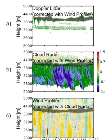
After subtraction of the vertical velocities measured by the wind profiler at the corresponding time and height interval, the true fall speed of the particles relative to the air becomes visible (see Fig. 10 and compare with Fig. 8). After this cor-rection, fall streaks in the virgae are more coherent. Such a corrected fall velocity yields important information about particle size and shape. It could be used, for example, to de-rive the particles maximum diameter with methods such as those presented by (Mitchell, 1996; Heymsfield and West-brook, 2010).
The wind-profiler vertical velocities itself are corrected by spectral separation of the wind-profiler and the cloud-radar spectra in order to remove the particle influence from the wind profiler measurements and get the pure vertical-wind information, similar to the method proposed by Gage et al. (1999). A detailed description of this method will be given elsewhere (paper in preparation). In the highly turbulent re-gions of the liquid cloud layers the mutual correction tween Doppler lidar, cloud radar and wind profiler fails, be-cause the temporal and spacial resolution of the cloud radar
and wind profiler are not sufficient to resolve the small-scale turbulence.
Interesting to note is the sudden jump in fall velocity oc-curring at around 11:00 UTC. At this time, multiple turbulent layers are visible in the cloud radar at 3900 m and 4700 m. Particles produced by the upper layer may grow faster, rime or aggregate in the lower layer and therefore show a higher fall speed compared to those before.
4 Summary
Figure 9. The vertical velocities (a) and their power spectra (b) are
shown, taken at the red lines indicated in Fig. 8. It is clearly visible that only the Doppler lidar is able to sense the inertial subrange, where its power spectrum is close to thef−5/3line. The advantage of the Doppler lidar is also visible in (a), where fast changes of vertical velocity on time scales smaller than 10 s are visible only in the Doppler lidar measurements (red).
5 Conclusion and discussion
The combined vertical-velocity measurements yield unique information about the movements of small and big particles together with the true movement of the air. In the corrected particle fall velocities, systematic errors of about 0.3 m s−1 have been detected (see Fig. 7). This corresponds to the ac-curacy of the single instruments which is on the order of 0.1 m s−1. The big pulse volume of the wind profiler obvi-ously poses problems if the small-scale variability is high, e.g., at turbulent cloud tops.
It was shown that the use of a wind profiler can fill the white spaces left on the vertical-velocity picture drawn by Doppler lidars and cloud radars. On the other hand, a Doppler lidar can detect cloud and aerosol particles, where cloud radar and wind profiler are not sensitive enough. Large-scale atmospheric motion becomes visible together with clouds and the extent and strengths of vertical-velocity fields can be studied independent of the presence of tracers, like aerosol particles or cloud droplets.
V
er
tical
V
el
ocity [
m
s
⁻
¹]
He
ig
ht
[m
]
He
ig
ht
[m
]
He
ig
ht
[m
]
Doppler Lidar
(corrected with Wind Profiler)
Cloud Radar
(corrected with Wind Profiler)
Wind Profiler
(corrected with Cloud Radar)
a)
b)
c)
Figure 10. Demonstration of mutual vertical-velocity correction of
the measurement shown in Fig. 8. A nearest-neighbor interpolation of the wind-profiler data was subtracted from the cloud-radar and Doppler lidar vertical velocities. The Doppler lidar is used to iden-tify liquid layers (gray area). Inside and above these layers the sub-traction procedure might be invalid because of several effects in-cluding liquid attenuation and small-scale turbulence that cannot be resolved by the wind profiler.
Acknowledgements. The research leading to these results has
received funding from the European Union Seventh Framework Programme (FP7/2007-2013) under grant agreement no. 262254.
Edited by: A. Stoffelen
References
Angevine, W. M.: Errors in Mean Vertical Velocities Measured by Boundary Layer Wind Profilers, J. At-mos. Ocean. Tech., 14, 565–569, doi:10.1175/1520-0426(1997)014<0565:EIMVVM>2.0.CO;2, 1997.
Böhme, T., Hauf, T., and Lehmann, V.: Investigation of short-period gravity waves with the Lindenberg 482 MHz tropo-spheric wind profiler, Q. J. Roy. Meteor. Soc., 130, 2933–2952, doi:10.1256/qj.03.179, 2004.
Bühl, J.: Combined lidar and radar observations of vertical motions and heterogeneous ice formation in mixed-phase layered clouds, Univ. Leipzig, available at: http://nbn-resolving.de/urn:nbn:de: bsz:15-qucosa-171998, 2015.
Bühl, J., Engelmann, R., and Ansmann, A.: Removing the laser-chirp influence from coherent doppler lidar datasets by two-dimensional deconvolution, J. Atmos. Ocean. Tech., 29, 1042– 1051, doi:10.1175/JTECH-D-11-00144.1, 2012.
for-mation with lidar/radar: comparison of CALIPSO/CloudSat with ground-based observations, Geophys. Res. Lett., 40, 4404–4408, doi:10.1002/grl.50792, 2013.
Chandra, A. S.,Kollias, P., Giangrande, S. E., and Klein, S. A.: Long-Term Observations of the Convective Boundary Layer Us-ing Insect Radar Returns at the SGP ARM Climate Research Fa-cility, J. Climate, 23, 5699–5714, doi:10.1175/2010JCLI3395.1, 2010.
Gage, K. S., Williams, C. R., Ecklund, W. L., and John-ston, P. E.: Use of two profilers during mctex for unam-biguous identification of bragg scattering and rayleigh scat-tering, J. Atmos. Sci., 56, 3679–3691, doi:10.1175/1520-0469(1998)055<2974:EREFSW>2.0.CO;2, 1999.
Geerts, B. and Miao, Q.: The Use of Millimeter Doppler Radar Echoes to Estimate Vertical Air Velocities in the Fair-Weather Convective Boundary Layer, J. Atmos. Oceanic Technol., 22, 225–246, doi:10.1175/JTECH1699.1, 2005.
Görsdorf, U., Lehmann, V., Bauer-Pfundstein, M, Gerhard, P., Dmytro, V., Vladimir, V., and Vadim, V.: A 35-GHz polarimet-ric doppler radar for long-term observations of cloud parameters – description of system and data processing, J. Atmos. Ocean. Tech., 32, 675–690, doi:10.1175/JTECH-D-14-00066.1, 2015. Heymsfield, A. J. and Westbrook, C. D.: Advances in the
Estimation of Ice Particle Fall Speeds Using Laboratory and Field Measurements, J. Atmos. Sci., 67, 2469–2482, doi:10.1175/2010JAS3379.1, 2010.
Hocking, W. K.: On the extraction of atmospheric turbulence pa-rameters from radar backscatter Doppler spectra – I. Theory, J. Atmos. Terr. Phys., 45, 89–102, 1983.
Illingworth, A. J., Hogan, R. J., O’Connor, E. J., Bouniol, D., De-lanoë, J., Pelon, J., Protat, A., Brooks, M. E., Gaussiat, N., Wil-son, D. R., Donovan, D. P., Baltink, H. K., van Zadelhoff, G.-J., Eastment, J. D., Goddard, J. W. F., Wrench, C. L., Haeffe-lin, M., Krasnov, O. A., Russchenberg, H. W. J., Piriou, J.-M., Vinit, F., Seifert, A., Tompkins, A. M., and Willén, U.: Cloudnet, B. Am. Meteorol. Soc., 88, 883–898, doi:10.1175/BAMS-88-6-883, 2007.
Knight, C. A. and Miller, L. J.: Early radar echoes from small, warm cumulus: Bragg and hydrometeor scatter-ing, J. Atmos. Sci., 55, 2974–2992, doi:10.1175/1520-0469(1999)056<3679:UOTPDM>2.0.CO;2, 1998.
Korolev, A. and Field, P. R.: The effect of dynamics on mixed-phase clouds: theoretical considerations, J. Atmos. Sci., 65, 66, doi:10.1175/2007JAS2355.1, 2008.
Lane, S. E., Barlow, J. F., and Wood, C. R.: An assessment of a three-beam Doppler lidar wind profiling method for use in urban areas, J. Wind Eng. Ind. Aerod., 119, 53–59, doi:10.1016/j.jweia.2013.05.010, 2013.
Lehmann, V.: Optimal Gabor-Frame-Expansion-Based Intermittent-Clutter-Filtering Method for Radar Wind Profiler, J. Atmos. Oceanic Technol., 29, 141–158, doi:10.1175/2011JTECHA1460.1, 2012.
Luke, E. P., Kollias, P., and Shupe, M. D.: Detection of supercooled liquid in mixed-phase clouds using radar Doppler spectra, J. Geophys. Res.-Atmos., 115, 2156–2202, doi:10.1029/2009JD012884, 2010.
Mitchell, D. L.: Use of mass- and area-dimensional power laws for determining precipitation particle terminal veloc-ities, J. Atmos. Sci., 53, 1710–1723, doi:10.1175/1520-0469(1996)053<1710:UOMAAD>2.0.CO;2, 1996.
Päschke, E., Leinweber, R., and Lehmann, V.: An assessment of the performance of a 1.5 µm Doppler lidar for operational vertical wind profiling based on a 1-year trial, Atmos. Meas. Tech., 8, 2251–2266, doi:10.5194/amt-8-2251-2015, 2015.
Pearson, G., Davies, F., and Collier, C.: An Analysis of the Per-formance of the UFAM Pulsed Doppler Lidar for Observing the Boundary Layer, J. Atmos. Ocean. Tech., 26, 240–250, doi:10.1175/2008JTECHA1128.1, 2009.
Protat, A. and Williams, C. R.: The accuracy of radar estimates of ice terminal fall speed from vertically pointing Doppler radar measurements, J. Appl. Meteorol. Clim., 50, 2120–2138, doi:10.1175/JAMC-D-10-05031.1, 2011.
Simmel, M., Bühl, J., Ansmann, A., and Tegen, I.: Ice formation in altocumulus clouds over Leipzig: Remote sensing measure-ments and detailed model simulations, Geophys. Res. Abstr., EGU2014-6500, EGU General Assembly 2014, Vienna, Austria, 2014.
Strauch, R. G., Merritt, D. A., Moran, K. P., Earnshaw, K. B., and De Kamp, D. V.: The Colorado wind-profiling net-work, J. Atmos. Ocean. Tech., 1, 37–49, doi:10.1175/1520-0426(1984)001<0037:TCWPN>2.0.CO;2, 1984.
Tridon, F., Battaglia, A. Kollias, P., Luke, E., and Williams, C. R.: Signal Postprocessing and Reflectivity Calibration of the Atmospheric Radiation Measurement Program 915-MHz Wind Profilers, J. Atmos. Ocean. Tech., 30, 1038–1054, doi:10.1175/JTECH-D-12-00146.1, 2013.
Wandinger, U., Seifert, P., Engelmann, R., Bühl, J., Wagner, J., Schmidt, J., Pospichal, B., Baars, H., Hiebsch, A., Kanitz, T., Skupin, A., Pfitzenmaier, L., Heese, B., Althausen, D., and Ans-mann, A.: Observations of aerosol-cloud-turbulence interaction with integrated remote-sensing instrumentation, 9th International Symposium on Tropospheric Profiling (ISTP), L’Aquila, Italy, 3– 7 September 2012.
Weber, B. L. and Wuertz, D. B.: Comparison of rawin-sonde and wind profiler radar measurements, J. At-mos. Ocean. Tech., 7, 157–174, doi:10.1175/1520-0426(1990)007<0157:CORAWP>2.0.CO;2, 1990.
Woodman, R. F. and Guillen, A.: Radar Observations of Winds and Turbulence in the Stratosphere and Meso-sphere J. Atmos. Sci., 31, 493–505, doi:10.1175/1520-0469(1974)031<0493:ROOWAT>2.0.CO;2, 1974.
Zhang, D., Wang, Z., and Liu, D.: A global view of midlevel liquid-layer topped stratiform cloud distribution and phase partition from CALIPSO and CloudSat measurements, J. Geophys. Res.-Atmos., 115, D00H13, doi:10.1029/2009JD012143, 2010. Zhang, Y., Klein, S. A., Boyle, J., and Mace, G. G.: