Journal of
Applied Research on Industrial Engineering
Journal of Applied Research on Industrial Engineering
Vol. 1, No. 3 (2014) 180-197
1.
Introduction
In today's business world, a company needs its own supply chain and logistics management to be able to effectively compete with other companies. In other words, supply chain management (SCM) and logistics tasks can be outlined, as such maximizing the added value and reducing total cost during
* Corresponding Author: Farhad Yazdani ([email protected])
A bi-objective mathematical model for designing the closed-loop
supply chain network with disruption in production centers
Farhad Yazdani
1,*, Reza Tavakkoli-Moghaddam
2, Mahdi Bashiri
31 Department of Industrial Engineering, Najafabad Branch, Islamic Azad University, Isfahan, Iran ([email protected]) 2 School of Industrial Engineering, University of Tehran, Tehran, Iran ([email protected])
3 Department of Industrial Engineering, Shahed University, Tehran, Iran, Iran ([email protected])
a r t i c l e i n f o a b s t r a c t
Article History:
Received: 19 September 2014 Received in revised format: 2 October 2014
Accepted: 5 October 2014 Available online: 9 October 2014
Keywords:
Bi-objective model,
Closed-loop supply
chain network,
Facility disruptions.
181
the business processes with a focus on speed and response to market needs. Nowadays, SCM andlogistics have become a requirement, especially for manufacturing industries that wish to supply their products at competitive costs and higher quality than their competitors. Reverse logistics models can be divided into two categories: (i) issues that focus only on the recursive network and (ii) issues that a recursive network has been integrated with the forward network. Regarding the issues of the first category, the point which is of great importance is that these issues may be affected by sub-optimization. Therefore, in recent years, the researchers’ focus has been higher on the issues of the second category. Considering the mentioned items, in this study, a closed-loop model has been considered that in addition to maximizing the profit reduces the delivery time to customers. This model is studied in the multi-product and single-period mode, in which all the demands of the customers are met. In continuation, initially, an overview of works done in this field will be examined and in the following sections network modeling is provided and by using the proposed solution, the model is solved. Finally, the results obtained from solving the model and the conclusions are presented.
2.
Literature Review
Much of the literature in the field of the logistic network design consists of different facility location models on the basis of the mixed-integer linear programming. These models consists of a variety of simple models (e.g., facility location models with the unlimited capacity) up to more complex models (e.g., multilevel models with limited capacity) or multi-commodity models. Also, strong algorithms on the basis of the theory of combinatorial optimization have been presented for solving these models. The models presented for the supply chain network design are discussed as follows. Salema et al. (2010) provided a multi-product and multi-period model for the supply chain network design and planning by reverse flows. To model their network, they used a graph approach on the basis of the traditional notions of nodes and arcs. They performed the strategic design of the supply chain along with a practical plan, which covered supply, production, storage and distribution sections. El-Sayed et al. (2010) developed a multi-period and multi-level reverse-forward logistics network design model. Their model possess a 3-level network in the forward direction (i.e., suppliers, facilities and distribution centers), and two levels in a reverse direction (i.e., montage and collection centers). In this paper, the customers are divided into two categories: primary consumers and secondary consumers. Primary customers’ demands have been considered as probable demands and secondary customers’ demands have been considered as definitive demands. The model presented by them is a mixed-integer linear programming model that maximizes the expected profit.
182
total fixed costs and transportation costs are minimized. In this model, uncertainty has beenconsidered that includes parameters of returned products, the demand for recycled products and transportation costs. For modeling the uncertainty, they have used the randomized programming.
Amin and Zhang (2012) examined a closed-loop supply chain network that includes manufacturing, montage, repair and renovation, and disposal places. Their work is divided into two phases. In the first phase, a framework is provided to identify supplier selection criteria. Then a fuzzy approach is designed for the selection of suppliers in order to determine the weight of suppliers. In the second phase, a multi-objective mixed-integer linear programming model is presented. In this model, the profit and the total value are maximized and the number of purchased defective items is minimized. Tabrizi and Razmi (2013) presented a mixed-integer nonlinear fuzzy model for risk management in the supply chain network design providing a mixed-integer nonlinear mathematical model. To consider the uncertainty conditions, they used a fuzzy set theory and in order to solve their model they applied a Benders Decomposition method. By the sensitivity analysis and providing numerical examples, they evaluated their proposed model. Amin and Zhang (2012) presented a multi-objective location model for closed-loop supply chain networks under uncertainty of demand and provided a mixed-integer linear programming model that minimizes the total cost. They also examined the impact of the uncertainty of demands and returns on the form of the network by contingency planning. Ramezani et al. (2013) presented a multi-objective probabilistic model under conditions of uncertainty, which has three levels in the forward direction (i.e., suppliers, manufacturing and distribution centers), and two levels in reverse direction (i.e., collection and disposal). Among the used uncertain parameters, we can refer to price of products, production and operating costs, demand and return rates, which are defined by a number of scenarios. In their proposed model, the objective is to maximize profit, customer responsiveness and quality of purchased raw material from the supplier. Also, financial risk has been calculated for relative valuation of the objectives.
In addition to designing a reverse-forward supply chain network, Keyvan Shokooh et al. (2013) applied dynamic pricing for returned products. Their model is a level, period and multi-product model, in which the returned multi-products are classified according to their quality and a different price is provided for each category. The sole purpose of the model is to minimize the costs, which include fixed costs, operating and maintenance and purchase cost of returned products. For solving their model, they presented a mixed-integer linear programming model. The results indicate that the use of dynamic pricing instead of static pricing and linear pricing approach for these models provided an acceptable answer. Arabzad et al. (2014) proposed a multi-objective optimization algorithm for solving a new multi-objective location-inventory problem in a distribution center (DC) network with the presence of different transportation modes and third party logistics (3PL) providers. In this model, 3PL is responsible to manage inventory in DCs and deliver products to customers. Furthermore, they proposed a non-dominated sorting genetic algorithm (NSGA-II) to perform high-quality search using two-parallel neighborhood search procedures for creating initial solutions. The potential of this algorithm evaluated by its application to the numerical example. Then, the obtained results are analyzed and compared with multi-objective simulated annealing (MOSA).
183
conditions of uncertainty. Their model consistently designed the intended network by employing anefficient and reliable approach. The network provided by them is a level, facility, multi-product and multi-provider network. To solve the proposed model, a new interactive hybrid approach is developed by combining a number of effective approaches in the past. This method is a fuzzy two-objective mixed-integer linear programming model. To get closer to the real world results a case study on the iron factory is considered. Finally, the results obtained from solving the model are provided to demonstrate the applicability and accuracy of the proposed model. Ghorbani et al. (2014) considered a fuzzy goal programming approach for solving a multi-objective model of the reverse supply chain design. This model involves of three objectives that minimizes the recycling cost, rate of waste generated by recyclers and material recovery time in such a way that the best set of recyclers to allocate products is determined. The main contribution of the proposed model is to consider the cost, time and efficiency rate to design a responsive and efficient reverse supply chain. A numerical example is conducted to validate the model.
Hatefi et al. (2014) presented a model for designing an integrated supply chain network. In their model, they used the concepts of reliability to evaluate the damaged facilities. In their model, the facilities are divided into two categories of reliable and unreliable facilities and unreliable facilities lose part of their capacity in the event of disruption. Therefore, in order to meet customer demand, a part of the demand is supplied by the residual capacity and part of it is supplied by sharing strategy, in such a manner that goods are carried from reliable facilities to unreliable facilities. This model is a single-product and multi-level model and production and recycling and collection and distribution centers are considered as a combination. The objective function consists of minimizing the fixed costs, transportation, operating and disruption costs in facilities. Parameters of the demand and return rates of product, transportation costs, fixed costs, operational costs and the capacity of facilities are considered in a fuzzy form. To deal with the uncertainty, reputation-based imposed math program is employed. Finally, to validate the model, numerical examples of solutions and the sensitivity analyzes were performed.
Pishvaee et al. (2014) presented a multi-objective location programming model to design the supply chain network for the pharmaceutical industry. Their proposed model is a stable model that consists of the triple economic, environmental (green) and social objectives. Economic objective includes minimizing the fixed costs, operating and transportation costs and environmental objective includes minimizing the environmental impact of transportation and operational activities and the social purpose includes maximizing created jobs and local development and to minimize the risk of consumers and workers injuries. To solve the model, the accelerated Benders Decomposition algorithm was used. Ramezani et al. (2014) presented a multi-product and multi-period model for designing a closed-loop supply chain network under fuzzy environment. In their network, the movement of goods between facilities of two levels can be performed by different transport models. Their proposed model consists of four layers in the forward direction (i.e., supplier, manufacturer, distribution centers and customers) and three layers in reverse order (i.e., customers, collection and disposal centers). Their model includes three objectives. The first objective is to maximize profit that this objective becomes possible by maximizing difference between revenues and costs. The second purpose is to maximize the level of servicing. This goal is achieved by minimizing the transportation time in forward and reverse direction. The third objective maximizes a sigma quality level that this goal is performed by minimizing the number of defective raw materials produced by the supplier. In this way, the quality of the parts produced in manufacturing centers will increase.
184
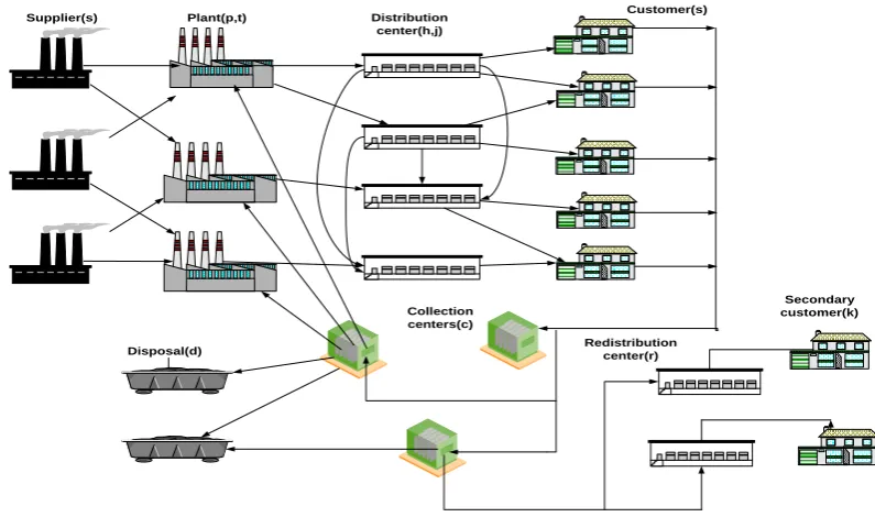
The proposed network in this study has three levels in the forward direction (i.e., suppliers,producers and distributors) and three levels in reverse direction (i.e., collection, redistribution and disposal centers). Initially, the manufacturing factories provide their needed raw materials from the suppliers. Final products manufactured in production centers are sent to distribution centers. Then the products are delivered to customers upon their request. In this network, each customer is allowed only to receive a product from one distribution center. In order to return, a percentage of these products are collected from customers by collecting centers. In the collection centers, initially the returned products are inspected, and then those products that are reproducible are again transferred to the manufacturing factories. Some of the products that are no longer usable are sent to disposal centers. Other products that have lost their initial quality but are still reusable are sent to distribution centers to be sent to the secondary customers. Facilities in the supply chain can be disrupted due to a variety of reasons (e.g., natural and humanitarian disasters), and cannot be able to work with their intended capacity. These facilities either completely lose their capacity or only a fraction of this capacity is disrupted and the intended facility can continue to operate with the remaining capacity.
In this research, production centers are divided into two reliable and unreliable categories. Reliable production centers, typically manufacture with the available capacity and the required product is sent to distribution centers; however, unreliable centers may be disrupted with certain probability. If an unreliable center becomes disrupted, it will lose some of its capacity. Therefore, it will not be capable of answering the needs of its distribution centers. In this study, to deal with such problems, a sharing strategy is used. This means that, if an unreliable production facility does not meet the needs of its distribution center, this distribution center would provide the remaining of its requirements from other distributors who receive products from reliable production centers. Fig. 1 shows a configuration of the proposed network and the flow of products between different facilities. After configuring the network, a mathematical model is proposed considering a multi-product and bi-objective one. The first objective is to maximize the expected profit of the network. This objective is achieved from the difference between the proceeds from the sale of products to primary and secondary customers and costs, which include variable costs (e.g., purchase cost, transportation costs, manufacturing costs, distribution costs, collection costs, operating costs and fixed costs of constructing facilities). The second objective maximizes the level of servicing to customers that this objective is achieved from weighted sum of the forward and reverse flows.
3.1.
Model decisions
Some of the decisions made in the proposed model are as follows: 1) Determining the location of each facility
2) Determining the number of reliable and unreliable production centers
3) Determining the amount of purchased raw materials and products among facilities
3.2.
Model assumptions
In the proposed supply chain network design problem, the following assumptions are considered in the model:
1) The proposed model is a multi-product and single-period model. 2) The location of suppliers and customers is known and constant.
3) Potential sites for factories, distributors, and collection and disposal centers are known. 4) Each customer can only get product from one distribution center.
185
6) The flow of products can only be established between facilities of two successive levels ofnetwork layers. Also at the level of distributors, the product flow can occur in the same facilities.
7) Uncertainty is considered for some parameters of the model.
8) The quality level of the products sent to secondary customers is lower than primary products and they are sold at cheaper prices.
Supplier(s) Plant(p,t) Distribution center(h,j)
Customer(s)
Disposal(d)
Collection centers(c)
Secondary customer(k) Redistribution
center(r)
Fig. 1. Proposed closed-loop logistic network
Sets, parameters and variables of the model are described below:
3.3.
Sets
S: Set of fixed locations of suppliers (s = 1, 2..., S)
P: Set of potential sites of the trusted factories (p = 1, 2..., P)
T: Set of potential sites of unreliable factories (t = 1, 2..., T)
H: Set of potential locations of distribution centers (these centers receive products from the P
production center) (h = 1, 2..., H)
J: Set of potential locations of distribution centers (these centers receive products from the T
production center) (j = 1, 2..., J)
I: Set of potential locations of collection centers (i = 1, 2..., I)
D: Number of potential sites of the disposal centers (d = 1, 2..., D)
C: Set of fixed locations of the primary customers (c = 1, 2..., C)
K: Set of fixed locations of the secondary customers (k = 1, 2..., K)
186
M: Set of raw materials (m = 1, 2..., M)
3.4.
Parameters
Demands:
DCL : Demand of the primary customer c for product L
Variable costs:
Pcl : Unit price of the sale of L product to customer C
PKL : Unit price of the sale of L product to secondary customer K
PSM : Unit cost of purchasing raw material M from the supplier S
PP pl = PP tl: the unit cost of production of the product L in the factory (p and t)
CPH = CPJ unit cost of distribution and operations at the distribution center (h and j)
CI i : Unit testing and inspection cost collection center i
CD d : Unit cost of disposal at the disposal center d
CB t = CB pl: Unit cost of product recovery at the factory (p and t)
CR r : Unit cost of distribution at redistribution center r
Fixed costs:
FCPR p : Fixed costs of construction of reliable manufacturing factory p
FCPU t : Fixed costs of construction of unreliable manufacturing factory (FCPUt≤ FCPRp)
FCH h = FCJ j: fixed cost of construction of distribution center (h, j)
FCC i : Fixed cost of constructing collection center i
FCD d: Fixed cost of constructing disposal center d
FCR r : Fixed cost of construction of redistribution center r
Transportation costs:
TC spm : Unit cost of transporting raw material m from supplier s to factory p
TC stm : Unit cost of transporting raw material m from supplier s to factory t (TC spm=TC stm)
TC ph l: Unit cost of transporting product l from the factory p to the distribution center h
TC tjl : Unit cost of transporting product l from the factory t to the distribution center j (TC tjl= TC phl)
TC hcl : Unit cost of transporting product l from distribution center h to customer c
187
TC cil : Unit cost of transporting returned product l from customer c to collection center i
TC ipl : Unit cost of transporting reproducible product l from collection center I to factory p
TC itl : Unit cost of transporting reproducible product l from collection center I to factory t (TCitl=
TCipl)
TC idl : Unit cost of transporting product l from collection center I to disposal center d
TC irl : Unit cost of transporting product l from collection center I to redistribution center r
TC rkl : Unit cost of transporting product l from redistribution center r to secondary customer k
Times
TIPH phl : Transportation time of each unit of product l from production center p to the distributor h
TITJ tjl : Transportation time of each unit of product l from production center t to the distributor j
(TITJtjl = TIPH phl)
TIHC hcl : Transportation time of each unit of product l from distribution center h to the customer c
TIJC jcl : Transportation time of each unit of product l from distribution center j to the customer c
(TIJC jcl = TIHC hcl)
TICI cil : Transportation time of each unit of product l from customer c to collection center i
TIIP ipl : Transportation time of each unit of product l from collection center I to production center p
TIIT itl : Transportation time of each unit of product l from collection center I to production center t
(TIIP ipl = TIIT itl)
Capacity of the facilities:
CAS sm : Capacity of supplier s for raw material m
CAP p : Factory capacity p
CAP t : Factory capacity t
CAD h : Capacity of distribution center h
CAD t : Capacity of distribution center t
CAC I : Capacity of collection center i
CAR p : Capacity of factory p for recovery of products
CAR t : Capacity of factory t for recovery of products
CAM d : Capacity of disposal center d
CAN r : Capacity of redistribution center r
188
RR : Rate of return of products used by customers
RC : Rate of reproduction
RD : Rate of disposal
UR ml : Rate of using raw material m in the product l
α : Weighting factor for the importance of the forward responsiveness
Put : Percentage of disturbance in unreliable production center t in the forward direction
Pu't : Percentage of disturbance in unreliable production center t in the reverse direction
Maximum number of facilities:
MP : Maximum number of factories p that can be constructed.
MT : Maximum number of factories t that can be constructed.
MD : Maximum number of distribution centers h that can be constructed.
MJ : Maximum number of distribution center j that can be constructed.
MC : Maximum number of collection centers that can be constructed.
MN : Maximum number of disposal facilities that can be constructed.
MR : Maximum number of redistribution centers that can be constructed.
Continuous variables:
QTYs,p,m : Amount of raw material r that supplier sends s to factory p.
QTYs,t,m : Amount of raw material r that supplier sends s to factory t.
QTYp, h, l : Amount of product l sent from factory p to distribution center h.
QTYt, j, l : Amount of product l sent from factory t to distribution center j.
QTYh, c, l : Amount of product l sent from distribution center h to customer c.
QTYj, c, l : The amount of product l sent from distribution center j to customer c.
QTY c, i, l : Amount of returned product l sent from customer c to collection center i.
QTY i, p, l : Amount of reproducible product l sent from collection center i to factory p.
QTY i, t, l : Amount of reproducible product l sent from collection center i to factory t.
QTY i, d, l : Amount of reproducible product l sent from collection center i to disposal centerd.
189
QTY r, k, l : Amount of reproducible product l sent from redistribution center r to the secondary
customer k.
Binary variables:
UX t : If unreliable production center t is constructed 1; otherwise, 0
RX p : If reliable production center p is constructed 1; otherwise, 0
Y h : If the distribution center h is constructed 1; otherwise, 0
Y j : If the distribution center j is constructed 1; otherwise, 0
Z i : If the collection center i is constructed 1; otherwise, 0
U d : If the disposal center d is constructed 1; otherwise, 0
CC hc : If distribution center h sends the product to the customer c 1; otherwise, 0
CC jc : If distribution center j sends the product to the customer c 1; otherwise, 0
CC ci : If the collection center I gets the returned product of the customer c 1; otherwise, 0
3.5.
Objective functions
The objective function of the problem includes the maximizing of the profit of the supply chain network as explained below:
1) ) (2) 2 Min (1 )
phl phl tjl tjl hcl hcl jcl jcl
p h l t j l h c l j c l
cil cil ipl ipl itl itl
c i l i p l i t l
f QTY TIPH QTY TITJ QTY TIHC QTY TIJC
QTY TICI QTY TIIP QTY TIIP
Maxhcl cl rkl kl
h c l r k l
spm spm stm stm phl phl tjl tjl
s p m s t m p h l t j l
hcl hcl jcl hcl cil cil ipl
h c l j c l c i l i p l
Z Income Cost
Income QTY P QTY P
Cost QTY TC QTY TC QTY TC QTY TC
QTY TC QTY TC QTY TC QTY T
iplitl itl idl idl irl irl rkl rkl
i t l i d l i r l r k l
hjl hjl spm sm stm sm phl pl
h j l s p m s t m p h l
tjl tl icl i cil i ipl
t j l i c l c i l l
C
QTY TC QTY TC QTY TC QTY TC
QTY TC QTY P QTY P QTY PP
QTY PP QTY CP QTY CC QTY
pli p
itl pl idl d rkl r
i t l i d l r k l
t t p p h h j j i r r d d
t p h j i r d
CR
QTY CR QTY CD QTY CR
FCPU UX FCPR RX FCH Y FCH Y FCC Z FCR V FCD U
190
The objective function of the problem is to maximize the expected profit of the network which isachieved from the difference between expected income from the sale and expenses related to the chain. Chain costs include the costs of shipping goods between facilities, variable costs of the supply of the suppliers, the cost of production in factories, processing costs at distribution centers, test and inspection costs at the collection centers, the cost of reproduction in factories, the cost of disposal at disposal centers and fixed costs of establishing facilities.
The second objective function is to maximize the level of servicing to customers. Considering Equation 2, the sum of the time at which the products manufactured in factory are obtained by customer through the distribution centers in a forward network and the sum of the time at which the products returned from customers through collection centers are sent to factory for recycling is minimized. As a result, servicing to customers is done in less time and the level of servicing will increase.
3.6.
Constraints
Balance Constraint 3) ) 4) ) 5) ) 6) ) 7) ) 8) ) 9) ) 10) ) 11) ) 12) ) 13) ) 14) ) 15) ) 16) ) , , , , , , , , 1spm ipl ml phl ml
s i l h l
stm itl ml pjl ml
t i l j l
phl hcl hjl
p c j
tjl hjl h jcl
t h c
hcl cl hc
jcl cl jc
hc jc
h j
QTY QTY UR QTY UR p m
QTY QTY UR QTY UR t m
QTY QTY QTY h l
QTY QTY Y QTY j l
QTY D CC h c l
QTY D CC j c l
CC CC
, 1 , , , ,cil cl ci
i
ci i
cil ipl itl idl irl
c p t d i
ipl itl cil
p t c
idl cil d c irl cil r c irl rkl i k c
QTY D RR CC c l
CC c
QTY QTY QTY QTY QTY i
QTY QTY QTY RC i l
QTY QTY RD i l
QTY QTY RS i l
QTY QTY r l
191
Constraints 3 and 4 state that at each reliable p and unreliable t production center, for each rawmaterial, the outflow from that factory to distribution centers cannot be more than the total inflow to the same factory from the suppliers and collection centers. Constraint 5 ensures that for each product, the total flow is sent from a reliable production center p to a distribution center h is equal to the total flow sent from this distribution center to other distribution centers j, and outflow from that center to its customers. Constraint 6 ensures that for each product the total flow sent from an unreliable production center t to a distribution center and the total flow sent from other distributors to this center is equal to the outflow sent from that distribution center to the customers. Constraints 7 and 8 show that the sum of the products sent from distribution centers should be equal to the demands of customers. Constraint 9 shows that customers have single source, this means that customers receive the product only from one distribution center. Constraint 10 shows that how the products returned from the customers is transferred to collection centers. Constraint 11 like the Constraint 12 shows that customers have single source in the reverse direction, in other words, the products returned from each customer is received by one collecting center. Constraint 13 indicates that all products sent from each collection center are equal to the sum of products that enter to this center. Constraints 14 and 15 show that how the products returned from the customers are transferred to collection centers, factories, dismantling and redistribution centers. Constraint 16 ensures that the total flow sent to each redistribution center is equal to outflow sent from this center to secondary customers.
Capacity constraint 17) ) 18) ) 19) ) 20) ) 21) ) 22) ) 23) ) 24) ) 25) ) 26) ) 27) )
Constraint 17 states that the sum of the raw material provided by suppliers cannot be greater than the total available capacity of the supplier. Constraints 18 and 19 ensure that the outflow of each reliable and unreliable factory cannot exceed the capacity of the relevant factory. Constraint 20 shows that the outflow from each distribution center h (the center which receives product form reliable production center) to other distribution centers j and the customer is limited to the capacity of related facilities. Constraint 21 shows that the outflow from each distribution center j (the center which receives the
.
(1 )
(1 ' )
spm sm pphl p p
h l
tjl t t t
j l
hcl hjl h h
c l j l
jcl j j
c l
hjl j j
h l
cil i i
c l
ipl p p
i l
itl t t t
i l
QT Y CA S s m
QT Y CA P RX p
QT Y CA P pu UX t
QT Y QT Y CA D Y h
QT Y CA D Y j
QT Y CA D Y j
QT Y CA C Z i
QT Y CA R RX p
QT Y CA R pu UX t
idl d d
i l
irl r r
i l
QT Y CA M U d
192
product of an unreliable production center t is limited to the capacity of the related facility. Constraint22 states that flow that enters into a distribution center from other distribution centers h should not exceed the capacity of this center. Constraint 23 ensures that the outflow from each collection center cannot exceed the capacity of the related facility. Constraints 24 and 25 state that the total outflow from each collection center to the reliable and unreliable production centers for reproduction could not be more than the reproduction capacity of the relevant factory. Constraint 26 states that the inflow to disposal centers is limited to the capacity of the relevant disposal center.
Maximum number of facility
28) ) 29) ) 30) ) 31) ) 32) ) 33) ) 34) )
Constraint 27 ensures that the amount of inflow to each redistribution center could not exceed the capacity of the relevant facility. Constraints 35 and 36 imply that the sum of the products which are sent from the collection centers to reliable and unreliable production centers for reproduction should not exceed the total amount of raw materials sent from suppliers to production centers. Constraints 37 and 38 state that the sum of the products sent from the collection centers to reliable and unreliable production centers for reproduction should not be more than the total flow from production center to distribution centers. Other Constraints 35) ) 36) ) 37) ) 38) )
Constraints (39) and (40) respectively indicate zero and one variables and non-negativity of the variables of the product transfer flow between facilities.
p p t t h h j j i h r r d d
X
MP
X
MT
Y
MD
Y
MJ
Z
MC
V
MR
U
MN
ipl ml spm
i l s m
ipl ml stm
i l s m
ipl phl
i l h l
ipl tjl
i l j l
QTY UR
QTY
p
QTY UR
QTY
t
QTY
QTY
p
QTY
QTY
t
193
39))
(40)
4.
Solution approach
The intended problem is a bi-objective logistics network design problem, in which for its analysis augmented ɛ-constraint approach is used. Suppose that i numbers of objective functions are a maximization type and j numbers of objective functions are a minimization type. The steps of the above method are as follows:
1) Initially optimal value of each function is achieved separately and without considering other objectives (Z p).
( 41 )
2) At this stage, the optimum solution for each function is placed in other functions and the value of the objective function is obtained. (Zn)
3) The value of r is obtained from the following equation:
p n
r
Z
Z
(42)4) An objective function is considered as the main objective function and for other objectives we consider the value of e to be equal with Znand we solve the following model for various e in order to obtain a set of Pareto solutions.
(43)
In the above model, i is the index of maximum functions and j is the index of minimum functions. A negligible and usually medial amount is chosen for (Mavrotas and Floris, 2013).
5.
Computational results
In order to demonstrate the applicability of the proposed model, a numerical example is presented in this section. In this example, the number of suppliers is 6, the number of potential sites for reliable
, , , , , , , , 0,1 , , , , ,
p t h j i d hc jc ci
X X Y Y Z U CC CC CC p t h j i d
, , , , , , , , , , , 0 , , , , , , , , , ,
spm stm phl tjl hcl jc cil ipl itl irl rkl idl
QTY QTY QTY QTY QTY QTY QTY QTY QTY QTY QTY QTY s p t h j c i r d m l
max ( )
min ( )
s.t.
i
j
f x
f x
x
X
3 2 1
2 3
max ( ( )
(
....
)
s.t.
( )
( )
,
p
p
i i i
j j j
S
S
S
f x
r
r
r
f x
S
e
f x
S
e
x
S Si
R
194
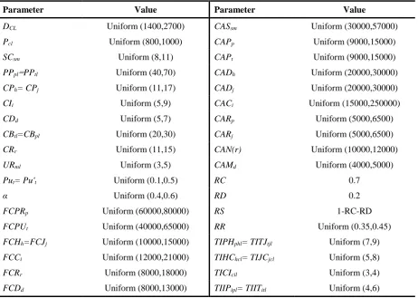
factories is 4 and for unreliable factories it is 5, by taking into account the percent of capacity lost as auniform distribution in the interval (0.1, 0.5), for distribution centers 4 and 3, for the collection centers 3, for disposal centers 4, for redistribution centers 3, the number of primary customers is 8 and the number of secondary customers is 2. Also the model is solved in a multi-product mode and by considering two products. Transportation costs are defined according to the distance between the facilities in the network. Other model parameters are shown in Table 1.
Table 1. Model parameters
Parameter Value Parameter Value
DCL Uniform (1400,2700) CASsm Uniform (30000,57000) Pcl Uniform (800,1000) CAPp Uniform (9000,15000) SCsm Uniform (8,11) CAPt Uniform (9000,15000) PPpl=PPtl Uniform (40,70) CADh Uniform (20000,30000) CPh= CPj Uniform (11,17) CADj Uniform (20000,30000) CIi Uniform (5,9) CACi Uniform (15000,250000) CDd Uniform (5,7) CARp Uniform (5000,6500) CBtl=CBpl Uniform (20,30) CARj Uniform (5000,6500) CRr Uniform (11,15) CAN(r) Uniform (10000,12000) URml Uniform (3,5) CAMd Uniform (4000,5000)
Put= Pu't Uniform (0.1,0.5) RC 0.7
α Uniform (0.4,0.6) RD 0.2
FCPRp Uniform (60000,80000) RS 1-RC-RD FCPUt Uniform (40000,65000) RR Uniform (0.35,0.45) FCHh=FCJj Uniform (10000,15000) TIPHphl= TITJtjl Uniform (7,9) FCCi Uniform (12000,21000) TIHChcl= TIJCjcl Uniform (5,8) FCRr Uniform (8000,18000) TICIcil Uniform (3,4) FCDd Uniform (8000,13000) TIIPipl= TIITitl Uniform (4,6)
195
Fig. 2. Profit versus Time6.
Sensitivity analysis
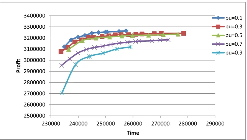
To study the behavior of the Pareto curve of profit and time towards the changes in percent of the lost capacity, this curve is drawn for different percentages. According to Fig. 3, the values of the Pareto curve are reduced by increasing the amounts of the lost capacity. This reduction is due to increased costs and reduced profitability of the network.
Fig. 3. Profit versus time perpercent of the lost capacity
3000000 3050000 3100000 3150000 3200000 3250000 3300000
230000 240000 250000 260000 270000 280000
Pr
o
fi
t
Time
2500000 2600000 2700000 2800000 2900000 3000000 3100000 3200000 3300000 3400000
230000 240000 250000 260000 270000 280000 290000
Pr
o
fi
t
Time
196
7.
Conclusion
In this study, a reliable multi-objective nonlinear mixed-integer programming model was provided for designing a forward-reverse logistics network against the risks caused by the disruption of facilities and risks related to uncertainty of parameters. To study disruption in facilities, two types of production centers were considered, reliable production centers which were stable and did not get damaged and unreliable production centers that in the event of disruption, the percentage of their capacity was lost. In this case, the distribution centers, which receive products from these centers, got deficient. This deficiency was compensated by other distribution centers. Objective functions of this model seek to maximize the profit and minimize the time (i.e., maximizing level of service). Among the main feature of this model, we could mention the ability to simultaneously adopt strategic and tactical decisions, its being multi-product, single-sourcing of customers and adopting decisions such as determining the location and time of establishing facilities, the rate of supply of raw materials from each supplier, the production rate of each of the units of production and distribution planning for the final product.The major contribution of this paper is to focus on considering reliability. In the proposed supply chain network, some plants were unreliable and in disruption condition were allowed to be partially disrupted and thus a percentage of their capacities might be lost. To compensate the lost capacity, a sharing strategy was considered. Furthermore, the second customer echelon was considered as a new echelon. To demonstrate the applicability and accuracy of the proposed model, a numerical example was presented, and by using the augmented ɛ-constraint approach, the Pareto curve for time against the profit was established that by using it the decision maker could choose his intended answer. This method had the ability to create a variety of efficient solutions. Also, in the sensitivity analysis, the impact of the lost capacity of unreliable production centers on the objective function of the problem was expressed.
For further research, the reader may consider the uncertain nature of the problem using a stochastic programming method (e.g., robust optimization and fuzzy programming). It is also possible to incorporate the reliability concepts into the transportation and inventory decisions to design a more reliable supply chain network. In addition, the proposed reliability concepts can be applied for supplier issues to cope with supplier disruptions. Modelling the different types of disruptions (caused by natural, man-made or technological threats) and their impacts on facilities and/or transportation links through a scenario-based approach will be of particular interest.
8.
References
Amin, S.H. and Zhang, G., (2012). “An integrated model for closed-loop supply chain configuration and supplier selection: Multi-objective approach”, Expert Systems with Applications, Vol. 39, No. 8, pp. 6782-6791.
Amin, S.H. and Zhang, G., (2013). “A multi-objective facility location model for closed-loop supply network under uncertain demand and return”, Applied Mathematical Modelling, Vol. 37, No. 6, pp. 4165-4176.
Arabzad, S.M., Ghorbani, M., andTavakkoli-Moghaddam, R. (2014).“An evolutionary algorithm for a new multi-objective location-inventory model in a distribution network with transportation modes and third-party logistics providers”.International Journal of Production Research, (In Press), pp. 1-13.
Demirel, N., Ozceylan, E., Paksoy, T. andGokcen, H., (2014). “A genetic algorithm approach for optimising a closed-loop supply chain network with crisp and fuzzy objectives”, International
197
El-Sayed, M., Afia, N. and El-Kharbotly, A. (2010).“A stochastic model for forward–reverselogistics network design under risk”, Computers & Industrial Engineering, Vol. 58, No. 3, pp. 423-431.
Ghorbani, M., Arabzad, S.M., andTavakkoli–Moghaddam, R. (2014).“A multi–objective fuzzy goal programming model for reverse supply chain design”, International Journal of Operational
Research, Vol. 19, No. 2, pp. 141-153.
Hatefi, S.M., Jolai, F., Torabi, S.A. and Tavakkoli-Moghaddam, R., (2014), “A credibility-constrained programming for reliable forward–reverse logistics network design under uncertainty and facility disruptions”, International Journal of Computer Integrated
Manufacturing, (In Press), (1-15).
Keyvanshokooh, E., Fattahi, M., Seyed-Hosseini, S.M., and Tavakkoli-Moghaddam, R., (2013). “A dynamic pricing approach for returned products in integrated forward/reverse logistics network design”, Applied Mathematical Modelling, Vol. 37, No. 24, pp. 10182-10202.
Mavrotas, G. and Florios. K. (2013), “An improved version of the augmented ε-constraint method (AUGMECON2) for finding the exact pareto set in multi-objective integer programming problems”, Applied Mathematics and Computation, Vol. 219, No. 18, pp. 9652-9669.
Pishvaee, M.S., Farahani, R.Z. andDullaert, W., (2010). “A memetic algorithm for biobjective integrated forward/reverse logistics network design”, Computers & Operations Research, Vol. 37, No. 6, pp. 1100-1112.
Pishvaee, M.S., Rabbani, M. andTorabi, S.A. (2011) “A robust optimization approach to closedloop supply chain network design under uncertainty”, Applied Mathematical Modelling, Vol. 24, No. 3, pp. 278-288.
Pishvaee, M.S., Razmi, J. and Torabi, S.A., (2014). “An accelerated Benders decomposition algorithm for sustainable supply chain network design under uncertainty: A case study of medical needle and syringe supply chain”, Transportation Research Part E: Logistics and
Transportation Review, Vol. 67, pp. No. 1, 14-38.
Ramezani, M., Bashiri, M. and Tavakkoli-Moghaddam, R. (2013). “A new multi-objective stochastic model for a forward/reverse logistic network design with responsiveness and quality level”, Applied Mathematical Modelling, Vol. 37, Nos. 1–2, pp. 328-344.
Ramezani, M., Kimiagari, A.M., Karimi, B. and Hejazi, T.H., (2014). “Closed-loop supply chain network design under a fuzzy environment”, Knowledge-Based Systems, Vol. 59, No. 1, pp. 108-120.
Salema, M.I., Barbosa-Póvoa, A.P., and Novais, A.Q. (2007). “A strategic and tactical model for closed-loop supply chains”, Estoril, Portugal: EURO Winter Institute on Location and
Logistics, Vol. 31, No. 3, pp. 361–386.
Tabrizi, B.H. and Razmi, J. (2013). “Introducing a mixed-integer non-linear fuzzy model for risk management in designing supply chain networks”, Journal of Manufacturing Systems, Vol. 32, No. 2, pp. 295-307.